S-classifications cells of 5, 10 and 15 orders of magnitude
Recall that the S-cells in our work are the scale intervals in which the scale class of systems under consideration exists.
The boundaries of these cells are defined by the intersections of the model sinusoid of SWS with the S-axis. These boundaries separate thirteen main scale classes of universal systems (see Fig. 1.7). Like any other boundaries, they possess their own width, and scale boundaries are no exception. They form vestigial, transitional regions along the S-axis, spanning a length of one order.
The objects located in these "vestibules" can be attributed both to the previous scale, or size class, and to the subsequent one. Therefore, if in the dimensional zones of the corresponding intersections of the S-axis with SWS it is possible to establish the presence of any disputable (from the classification point of view) objects, it will be an indirect evidence of objectivity of SWS-classification.
So, SWS is only a model, but are there limits to the size of objects in reality? To answer this question, it is necessary to consider an array of empirical data.
LET'S START WITH BIOSYSTEMS. Precisely because the data on the boundary sizes of biosystems are the best known to science among all the objects along the S-axis.
Even V.I. Vernadsky was interested in the question of size limits for living systems. He took a virus as the smallest particle of living things. This choice is far from accidental and still has scientific force. The point is that the most important feature of living, distinguishing it from non-living, is the ability to reproduce a copy of itself, which is impossible without DNA (or RNA). It is viruses that are the minimum possible living systems - "a small amount of genetic material (DNA or RNA) enclosed in a protective protein shell."33 Separately existing proteins are unable to reproduce, and there is no "naked", separately existing DNA or RNA in nature either.
The smallest virus known to science, tobacco mosaic virus (TMV), is 1.5 × \(10^{-6}\) cm in size.
Viruses were practically the first to be discovered in 1852 by the Russian botanist Dmitiri Ivanovsky.
The size of the largest virus known to science is 5.3 × \(10^{-6}\) cm.³⁴ We see that in terms of size, these objects fall within the size range of the transition class (\(10^{-5} \times 10^{-6}\) cm), between class five and six, where the S-axis intersects with the SWS. Our approach suggests that all objects in this size range belong to the transitional "vestigial" class.
This is why there are still debates about whether viruses should be considered living or non-living systems. After all, "viruses... have only some, but not all, of the features characteristic of living organisms."1 In particular, viruses cannot reproduce on their own; they need the environment of another, larger biosystem for this purpose.
So, since viruses are the smallest known protein-based living systems, we can define the lower dimensional limit for biosystems as \(10^{-5.5}\) cm (100–1000 angstroms).
Determining the size of the largest protein system, V.I. Vernadsky wrote: "The size of an organism is not accidental... The upper boundary is not accidental either: during the whole geological history it did not go beyond 200-300 m... we do not know the reason for it."2
V.I.Vernadsky does not specify in this work what kind of bio objects he had in mind. However, it is known that some species of whales have the highest size nowadays - 28 m. The remains of diplodocs3 have been found, which were about 30 m. in size. It is obvious that no animal reached the sizes indicated by V.I. Vernadsky. Most likely, he meant plants. Indeed, the height of sequoias4 can reach 110 m, brown algae up to 100 m long and lianas up to 240 m long are known.
If we convert these sizes into logarithms, we almost exactly get the upper limit for integral biosystems equal to \(10^{4.5}\) cm. Thus, all protein holistic systems occupy the size range from \(10^{-5.5}\) to \(10^{4.5}\) cm (see Fig. 1.11).
The length of this range on the S-axis is exactly equal to ten orders of magnitude!
Another surprising thing is also surprising. If we consider as biosystems also their all kinds of "clusters": herds, flocks, biocenosis and biosphere (as a functionally closed and integral system uniting everything), it turns out that they occupy five more orders on the S-axis.
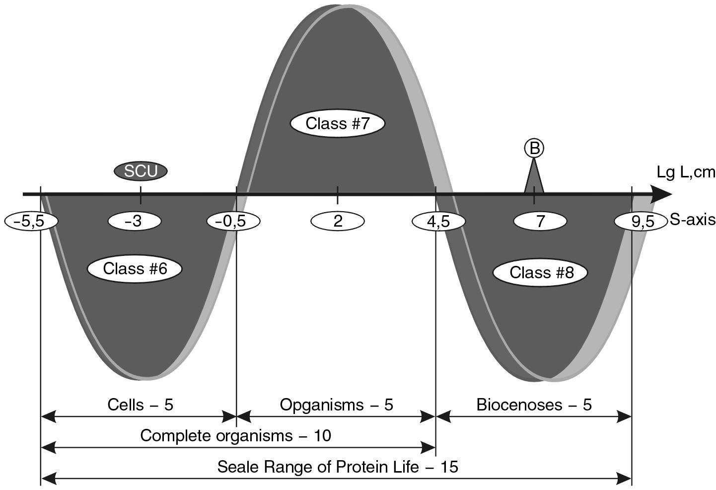
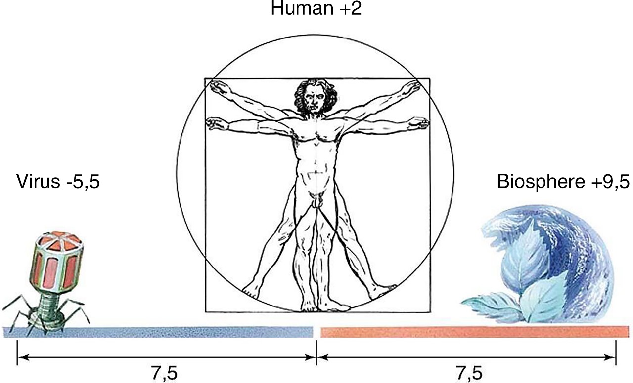
Fig. 1.12. Man by his size occupies the central place in the scale range of protein life on Earth. He is as many times larger than the smallest particle of life - virus, as many times smaller than the upper limit of life on Earth - Biosphere
After all, the "diameter" of the Biosphere is equal to the diameter of the Earth, including its atmosphere - 1.3 × \(10^{9}\) cm. If we take into account that viruses can survive outside the atmosphere, up to the magnetosphere, the size of the Biosphere reaches the theoretical classification boundary at the Stability Wave - \(10^{9.5}\) cm.
So, the whole scale range of protein life on the Earth occupies 15 = 10+5 orders of magnitude. Let us call this S-axis range the S-BIOLOGICAL SCALE DIAPASON (SBSD)
In the most general terms, the three intervals in the biological scale range can be labeled as cellular, organismal, and biocenosis scale classes of biosystems. The SBSD is divided into three areas (see Fig. 1.11) with five orders in each. The figure shows how clearly the dimensional boundaries of the classes commonly accepted in science coincide here with the boundaries of our model (points of intersection of the SWS with the S-axis).
The following scale structure (5+5)+5=15 can be distinguished on the example of consideration of the scale range of protein life. It can also be found in the scale ranges of other types of systems, as we will see in the future. This will serve as another confirmation that life is not something random in the Universe, since it is organized according to such global laws. So, the highest classification level is fifteen orders of magnitude. The boundaries of this scale interval determine the scale of existence of all forms of life in the Biosphere.
The next level is ten orders of magnitude, from viruses to algae in the Biosphere there are holistic organismal protein systems that have rigid internal structures, forms and contents.
Fundamentally different from them is the next largest class of protein systems, which occupies five orders of magnitude - these are biocenoses, which do not have rigid structures, forms and contents.
The same intervals on the S-axis, 5 orders of magnitude each, are occupied by cells - from viruses (\(10^{-5.5}\) cm) to large unicellular organisms (\(10^{-0.5}\) cm); and organisms - from primitive multicellular organisms (\(10^{-0.5}\) cm) to algae (\(10^{4.5}\) cm) (Fig. 1.11). Separately, it should be noted that man occupies on this scale interval of life an absolutely central position (see Fig. 1.12), since he is 7.5 orders of magnitude larger than viruses and the same number of orders of magnitude smaller than the Biosphere. We can speak all we want about the inadmissibility of anthropocentrism, but if in the HIERARCHICAL STRUCTURE OF THE BIOSPHERE HUMANITY occupies the CENTRAL PLACE, then this objective fact must be reckoned with. Let us consider to what extent the regularity revealed for biosystems is true for other large classes of objects of the Universe: stars, galaxies and atoms. Let us start with stars.
STARS (CLASS #9). According to the S - Wave of Stability - SWS model, all stars should be located in the scale interval \(10^{9.5}\)–\(10^{14.5}\) cm (Fig. 1.13). Let us see whether it is so in reality.
The diameter ranges for stars of different types can be determined from the data of the C. W. Allen handbook5:
- Supergiants - \(10^{12}\) to \(10^{14}\) cm;
- Giants - \(10^{11.5}\) to \(10^{12.5}\) cm;
- Dwarfs - \(10^{10}\) to \(10^{12}\) cm.
Thus, the size range for ordinary stars on the S-axis occupies 4 orders of magnitude from \(10^{10}\) to \(10^{14}\) cm. The mean scale value is \(10^{12}\) cm, which coincides exactly with the model stellar half-wave crest (see Fig. 1.7).
This range characterizes the bulk of stars. If we take into account that there are also very rare stars with smaller and larger (for example, the VV of Cepheus has a diameter of 4.7 × \(10^{14}\) cm.) sizes, the range can be extended in both directions by 0.5 orders of magnitude.
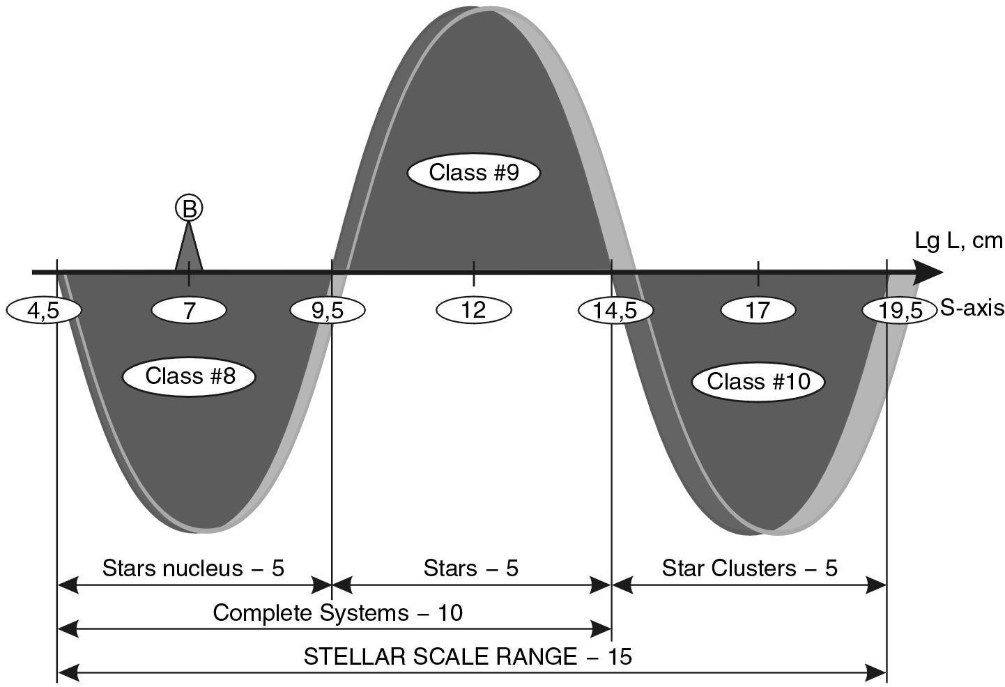
Fig. 1.13. Classification boundaries in the scale structure of the Universe
STAR SYSTEMS (CLASS #10). "Within the vast stellar system that is the galaxy, many stars are organized into smaller systems. Each of these systems can be thought of as a collective member of the galaxy. The smallest collective members of a galaxy are double and multiple stars. These are groups of two, three, four, etc. up to ten stars in which the stars are held close together by mutual attraction according to the law of universal gravitation"6. The larger collective members, which contain dozens or more stars, are clusters.
Stars in other galaxies also have the property of forming various systems from groups to clusters.
The distances in groups of stars are extremely different7: from close pairs (\(10^{12}\) cm) to wide pairs (\(10^{17}\) cm). There are two types of clusters: globular and diffuse. The diameters of scattered clusters8 range from \({6}\cdot{10^{18}}\) cm to \(10^{20}\) cm, and the number of stars in them from 20 to 2,000. Globular clusters have more stars: from \(10^{5}\) to \(10^{7}\), and their diameters range from \(10^{19}\) to \(10^{20}\) cm.
Thus, the extremely large star clusters have a size of \(10^{20}\) cm, which is exactly 10 orders of magnitude larger than the smallest stars.
It may seem that the author has arbitrarily limited stellar systems to clusters, since galaxies also consist of stars. However, the point is that a galaxy as a type of system differs from a star cluster in several fundamental respects.
- Star clusters do not have their own distinct structures (arms, disks, nuclei, halos, etc.). They are, figuratively speaking, swarms of stars, or colonies. Galaxies, like multicellular organisms, have their own life, which is not reducible to the combined functioning of individual stars.
- Star clusters are never found outside galaxies, although the sizes of some of them reach the size of dwarf elliptical galaxies. Galaxies, on the other hand, exist independently in outer space. To take an analogy. All systems are made up of atoms, but we clearly distinguish atomic assemblages in the form of a complex molecule or even a cell from a simple crystalline structure. Although galaxies are also ultimately made of atoms, it does not occur to us to call galaxies clusters of atoms.
In the following we will show that the boundary between star clusters and galaxies on the S-axis is common - it is the point of over S-axis cross-section with S - Wave of stability - SWS - \(10^{19.5 \pm 0.5}\) cm.
STAR NUCLEI (CLASS #8). Let us now consider the nuclear stars class. According to the S - Wave of stability - SWS model, it occupies the range from \(10^{4.5}\) to \(10^{9.5}\) cm. The characteristic point of the highest stability is the size of \(10^{7}\)- \(10^{8}\) cm (see Fig. 1.13).
The cores of stars can only be discussed theoretically, since even the core of the Sun, the closest star to us, has not yet been studied with instruments. However, since all stars sooner or later die, their remnants are always divided into two parts: outer and inner. The outer part, the envelope, collapses at different rates for stars of different masses. The inner part is compressed to a certain threshold, forming the dead (or dying) remnants of stars.
It can be conventionally assumed that these remnants are the nuclear formations of stars. They are divided mainly into three types: white dwarfs (WD), neutron stars (NS), and black holes (BH).
Small stars (with masses from 0.2 to 1.2 solar masses), shedding their envelopes, which gradually turn into planetary nebulae, become white dwarfs (WDs), whose sizes vary9 10 in the range of \(10^{8}\)-\(10^{10}\) cm.
More massive stars (with masses between 1.2 and 2.0 solar masses) explode as supernovae and their cores shrink to neutron stars (NSs), with average size estimates close to \(10^{7}\) cm.
The most massive stars (with masses greater than two solar masses) can form black holes (BHs) after the explosion; their sizes are estimated11 from \({3}\cdot{10^5}\) to \(10^{7}\) cm.
All of these objects are fundamentally different in their properties from ordinary stars. First, they no longer consist of atoms, but of their nuclei or elementary particles. Second, their radiation energy is no longer associated with thermonuclear synthesis, the main energy source of stars. The luminosity and color of these objects are also completely different from the luminosity and color of ordinary stars.
The bare nuclei of stars are a fundamentally different scale class (CLASS #8). Within this class, three types of bare nuclei occupy three regions:
- \(10^{5}\)-\(10^{7}\) cm - black holes (BHs);
- \(10^{7}\)-\(10^{8}\) cm - neutron stars (NS);
- \(10^{8}\)-\(10^{10}\) cm - white dwarfs (WD).
It is curious that the large-scale arrangement of stellar remnants on the S-axis mirrors the arrangement of the stars that produced them: the largest stars leave the smallest nuclei - BHs, and the smallest stars leave the largest of the nuclei - BCs.
So, the size limits for stellar nuclei occupy 5 orders of magnitude: from \(10^{5}\) to \(10^{10}\) cm. These limits are shifted relative to the model by 0.5 orders of magnitude to the right. The reason for this shift is probably due to the general rightward shift of all megamir dimensions, but we will consider this regularity further on. In general, the classification scheme for stars, like the biological scheme, consists of three intervals of 5 orders (see Fig. 1.13).
This range of 15 orders of magnitude can be called the stellar mass range, which is divided into three classes of 5 orders each: nuclear, stellar proper, and systemic stellar.
The above range characterizes the bulk of stars. If we take into account that there are also very rare stars with smaller and larger (For example, the VV of Cepheus has a diameter of 4.7 × \(10^{14}\) cm) sizes, the range can be extended in both directions by 0.5 orders of magnitude.
The reason for this shift is probably a general shift of all megaworld sizes to the right, but we will consider this regularity further on. In general, the classification scheme for stars, like the biological one, consists of three intervals of 5 orders (see Fig. 1.13).
This range of 15 orders of magnitude can be called the stellar scale range, which is divided into three classes of 5 orders of magnitude each: nuclear, stellar proper, and systemic stellar.
It should be noted that stellar pairs and groups (systems) actually begin with sizes of the order of \(10^{12}\) cm, which is 2.5 orders of magnitude to the left of their class boundary. However, this violation is apparent. After all, organisms also join into families, groups, herds and flocks, the sizes of which begin practically from the meter range (\(10^{2}\) cm). Which corresponds to the highest point of the crest of the wave of life (compare the two beginnings: for stars and for protein systems). Stars can form very close pairs too. This is a general systemic property to create all kinds of combinations of objects, and it does not depend on the size threshold.
We emphasize another thing: it was important for us to establish the size threshold to the left of which organisms (stars) could still exist on the S-axis, and to the right of which only their systems - biocenosis (star clusters) - can exist. Here we see that in the case of stars and in the case of organisms this threshold is modeled at the point of intersection of the right boundary of the middle class of the corresponding range with the S-axis (see Fig. 1.13).
Therefore, the interval of 15 orders of magnitude for both the Biosphere and the stars has an internal structure of 15 = 10+5 = (5+5)+5 and the same appearance: a central ridge and two half-waves on the left and right. This once again shows the fruitfulness of the wave model we have chosen.
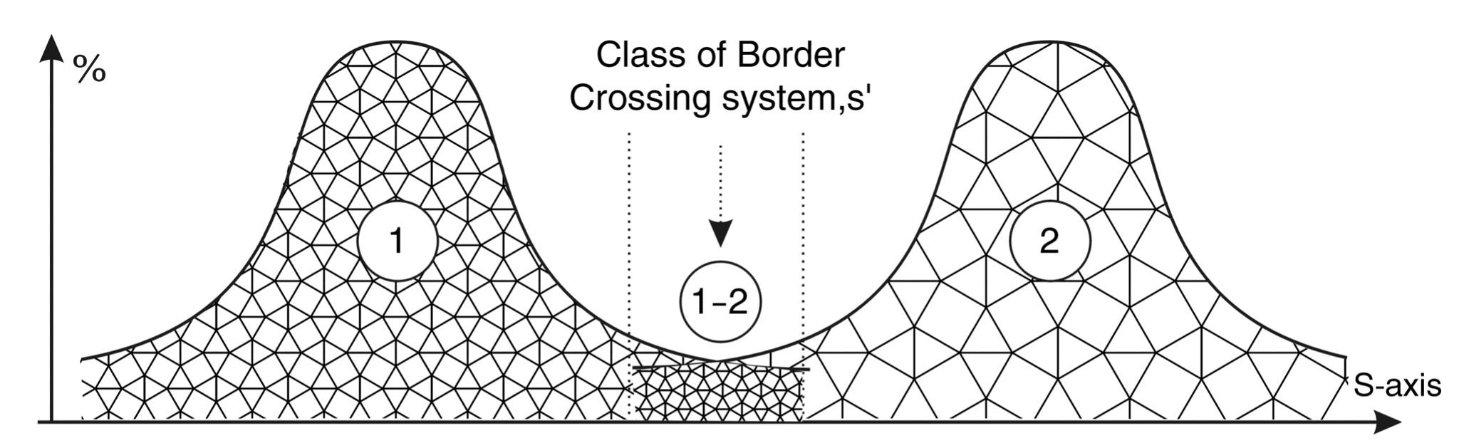 Fig. 1.14. Model of size distribution of objects in two boundary size classes. As a rule, there is a transition zone of one order of magnitude width at the boundary of classes, which is "populated" by disputable objects
So far we have considered scale intervals of classes. Let us now consider the boundary, for example, between two of them: No. 8 and No. 9. This will allow us to see the degree of accuracy of the S-classification proposed here.
We have already noted that astronomers do not find stars smaller than \(10^{10}\) cm. Such small stars are very difficult to see in the sky, so it is not excluded that it is still possible to meet a star whose size will be \(10^{9.5}\) cm. Especially since the determination of the diameters of stars is largely a theoretical rather than observational procedure. Consequently, we can PROPOSE that the point of intersection of the baseline SWS with the S-axis is the exact lower classification limit of the existence of stars.
A small methodological digression is necessary here. The point is that any classification boundary between neighboring classes in any parameter space, as we have already pointed out, is not a line but a strip. This means that there exists a region within such a parameter space in which one can find representatives shared by the class boundary (see Fig. 1.14).
The same is true for dimensions. Each of the neighboring classes has its own size range, the junction of these ranges represents a certain band on the S-axis - a Tambour Scale Interval of one order of magnitude. In such a tambour scale interval one can find both the largest representatives of the lower class and the smallest representatives of the upper class. It is almost obvious that the width of the transitional, vestigial class will depend on the sizes of the bordering classes. It is natural that for the analysis the selection of neighboring classes should be based on the principle of their identical scale extent.
Thus, for example, stars occur practically over 5 orders of magnitude. Their nuclei (white dwarfs, neutron stars and black holes) - also over 5 orders of magnitude. Hence, we are dealing with neighboring classes at scale levels. The boundary between these classes, as between any other classes, has a scale width of about 1 order of magnitude: from \(10^{9}\) to \(10^{10}\) cm, or \(10^{9.5 \pm 0.5}\) cm. This means that in this size range one can detect some stars that are almost not stars and some objects that are almost stars.
Consider, for example, the upper boundary of the nuclei of stars - white dwarfs, which, as we mentioned, have sizes differing by 2 orders of magnitude. The largest of them (\(10^{10}\) cm) "enter" an alien class - the stellar class. It is the largest of the white dwarfs, according to many astrophysicists, are in an intermediate state between stars and their cores. After all, it is in these stars that "hydrogen nuclear reactions occurring in a very thin spherical layer at the boundary of the dense degenerate matter of their interior and atmosphere,"12 are still going on.
The main energy of all white dwarfs is "only the result of the expenditure of thermal energy of atomic nuclei." Thus, large white dwarfs, which belong to the size range \(10^{9}\)-\(10^{10}\) cm, are intermediate transitional systems, because they, on the one hand, are exhausted stars. On the other hand, they partially continue to emit stellar (nuclear) energy. This fact confirms the correctness of the theoretically defined classification boundary between stars and their nuclei.
Besides this example, there is another fact that shows the reality of the size threshold between the two classes revealed in the model. It is interesting that this fact refers to completely different space systems - planets.
PLANETS (CLASS # 8). We only have the opportunity to study the planets of the solar system. Therefore, the statistical generalization we can make is not very representative. However, because of the importance of these astronomical bodies to us, we will still look at how their sizes are related to Stability Wave (SW).
The smallest independent planet is Mercury with a diameter of 0.38 × \(10^{9}\) cm, the largest is Jupiter, its diameter is just over \(10^{10}\) cm. According to the location of orbits around the Sun (inside or outside the asteroid ring), all planets can be subdivided into two groups:
Earth-group planets
- Mercury 0.485 × \(10^{9}\) cm
- Venus 1.210 × \(10^{9}\) cm
- Earth 1.276 × \(10^{9}\) cm
- Mars 0.679 × \(10^{9}\) cm
The planets of the Jupiter group
- Jupiter 1.426 × \(10^{10}\) cm
- Saturn 1.202 × \(10^{10}\) cm
- Uranus 0.490 × \(10^{10}\) cm
- Neptune 0.502 × \(10^{10}\) cm
- Pluto 0.640 × \(10^{9}\) cm
Between the orbits of these two groups there is an "empty" orbit filled with asteroids and rocks, which serves as a natural "natural boundary" separating the two types of planets. The laws of diameters of planetary orbits are a separate topic. Here we will turn to the fundamental physical difference between the planets of these two groups. Planets of the Earth group are solid bodies with a density greater than 2 g/cm3 (up to 5.5 g/cm3 ). The planets of the Jupiter group can be divided by physical properties into giant planets (gas balls with a density up to 2 g/cm3, close to the density of water) and the small solid planet Pluto.
If we arrange all the planets of the Solar System according to their sizes on the S-axis, they will occupy there two almost identical intervals of 0.5 orders of magnitude (see Fig. 1.15). Common for all solid planets is that their diameter does not exceed the value of \(10^{9.5}\) cm, the model boundary on the SW between dense nuclear formations and rarefied gaseous star formations. All planets in the Jupiter group are larger than this value -- except Pluto, and it is Pluto that is the exception in group II. It has a solid surface and a density greater than 2 g/cm3.
Here an interesting PROPOSITION arises. The fact is that Pluto is the outermost planet in the solar system. From Jupiter onward from the Sun, all planets are composed of light elements of the PERIODIC TABLE OF ELEMENTS (PTE) - all except Pluto, which is composed of heavy elements. This planet falls out of the general pattern of differentiation of protoplanetary cloud matter (light elements from outside the asteroid's ring) that many cosmogonic theories recognize. There is a problem with the appearance of Pluto's solid matter at the boundary of this gas region. We have to invent versions of Pluto's capture from other stellar systems.
However, we note that Pluto's physical properties do not fall out of the scaling pattern at all (see Fig. 1.15).
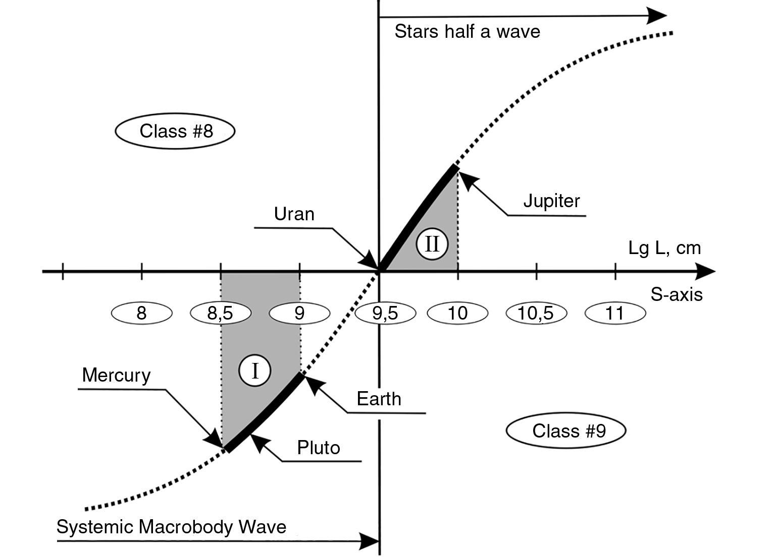 Fig. 1.15. S-classification of the planets of the Solar System. I - group of solid planets with density higher than 2 g/cm3. II - group of gaseous planets with density below 2 g/cm3. A scale periodicity of 0.5 orders of magnitude is evident
The question arises: is it a coincidence that the solar system is so organized that, regardless of orbit, all planets with sizes less than \(10^{9.5}\) cm are solids and those with sizes greater than \(10^{9.5}\) cm are gaseous (star-like)?
So, our PROPOSITION is reduced to the following: the place of a planet in three-dimensional space does not play the same essential role as its position in scale space. According to our model, if the size of the planet corresponds to the class of star nuclei, it is a solid bod. If its size refers to the class of stars themselves, it is a gaseous body.
Our model also reveals an additional regularity (see Fig. 1.15), which is very difficult to explain from the standpoint of the traditional theory of planetary formation in the solar system. It consists in the fact that the location of both groups of planets on the S-axis clearly shows 3 scaling intervals of about 0.5 orders of magnitude each. The first half-order is populated by planets of the Earth group (I) and Pluto, the second half-order is absolutely empty, the third half-order is populated by planets of the Jupiter group (II). The smallest planet of the Earth group - Mercury is close to the left boundary of the interval of Group I planets, i.e. to the S-axis point - 5 × \(10^{8}\) cm. The smallest of the gaseous planets of the Jupiterian group - Uranus is also close to the left boundary of the interval of group II planets, i.e. to the point of S-axis - 5 × \(10^{9}\) cm. Therefore, we can confidently assert that the left boundaries of the two planetary groups, according to empirical data, are located on the S-axis through one order of magnitude. Similarly, the largest planet of the inner group, the Earth, closes the interval I on the right, with its diameter 10 times smaller than that of Jupiter with an accuracy of 1%. Consequently, the right boundaries of intervals I and II on the S-axis are also 1 order of magnitude apart and with good accuracy.
Based on traditional approaches, how can the obvious fact that the sizes of the two types of planets occupy on the S-axis two intervals of 0.5 orders of magnitude with an empty gap between them of another 0.5 orders of magnitude be explained? Could the fact that the S-axis crosses the EI at the point where solid planets like the Earth no longer occur and gaseous, star-like planets like Jupiter begin be passed by?
Summarizing everything, we can PROPOSE that not only the planets of the Solar System, but also the planets of all systems of the Universe are divided into two classes similarly to the planets of the Solar System. And ALL PLANETS OF THE UNIVERSE WHICH SIZE IS LESS THAN \(10^{9.5}\) cm, WILL BE LIKE PLANETS OF THE EARTH GROUP, AND ALL PLANETS WHICH SIZE IS LARGER THAN THIS RANGE, WILL HAVE A GAS-BRASED COMPOSITION.
By the way, Jupiter emits 60% more energy than it receives from the Sun, which is why it is often called "almost a star". This is not surprising from the point of view of the classification boundaries of the Stability Wave, because in terms of its size it already belongs to the star class (CLASS #9: from \(10^{9.5}\) cm to \(10^{14.5}\) cm).
Our Earth is the largest planet of the first group, and its diameter is approaching star class. This, on the one hand, is remarkable, because it distinguishes it among other planets. However, it is worth considering whether there is no danger for the Earth in the fact that its size is very close to some transitional boundary of steady state for cosmic bodies. Thus, having examined "in a magnifying glass" one of the model classification boundaries, i.e., the point of intersection of the SW with the S-axis, we are convinced that it reflects quite well the real classification boundaries in the Universe.
Turning to the protein range, we recall that the dimensional boundary for the lower threshold of living systems is filled with viruses, which are still treated by various researchers as living or non-living systems. This indicates that this point of intersection of the SWS with the S-axis is also a real classification barrier for fundamentally different systems.
GALACTIC CLASSES #10, 11, 12. According to the SWS model, their objects occupy the interval from \(10^{14.5}\) to \(10^{28.2}\) cm (see Fig. 1.16). With \(10^{14.5}\) cm to \(10^{19.5}\) cm being the nuclear class, or the class of galaxy nuclei - and \(10^{19.5}\) cm to \(10^{24.5}\) cm being the class of galaxies themselves, or the structural class. Then come a few more orders, like star clusters and biocenoses, which should be filled with some non-rigid and open systems of galaxies.
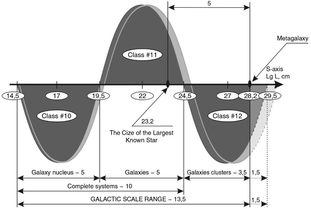 Fig. 1.16
Let us consider whether such a model division of the S-axis corresponds to the real difference in the properties of galaxy-class objects.
The total number of galaxies in the Metagalaxy is \(10^{10}\), which coincides surprisingly precisely with the main scale periodicity coefficient. The sizes of the most typical galaxies are enclosed in the range \(10^{21}\)-\(10^{23}\) cm 13. Hence, the average scale size for galaxies is \(10^{22}\) cm. Our own Galaxy belongs to very large systems. The diameter of its halo (a spherical cluster of tens of billions of stars) is \(10^{23}\) cm, and the thickness of the spiral disk is 15 times smaller: 6 × \(10^{21}\) cm 14.
Astronomers know several galaxies whose sizes are larger than ours: according to V. Zonn 15 - this is galaxy M101, its diameter is equal to 1.5 × \(10^{23}\) cm; according to B. A. Vorontsov-Velyaminov 16 - this is galaxy M31, its diameter is equal to 1.8 × \(10^{23}\) cm.
The mentioned sizes are the limit for the possible size of galaxies. Only hypergalaxies - several galaxies united by a common corona - have even larger sizes; B. A. Vorontsov-Velyaminov calls them "nests of galaxies". Their sizes, however, are not much larger than the specified limit; according to B. A. Vorontsov-Velyaminov, they do not exceed 3 × \(10^{23}\) cm.
Thus, on the S-axis, ordinary galaxies occupy only 2 orders of magnitude from \(10^{21}\) to \(10^{23}\) cm. If we go toward even larger scales, the nests of galaxies are followed in size by groups with an average size of \(10^{24}\) cm and clusters with an average size of \(10^{25}\) cm. Clusters are the limit for the galactic class of systems, for they can still be formed by the galaxies' own gravitational interaction. Beyond this threshold, the world of the Metagalactic substructure begins, the world of super clusters (\(10^{26}\) cm).
Let us now analyze the systems that are located on the S-axis to the left of the galactic "ridge." In the range \(10^{20}\)- \(10^{21}\) cm there are so-called dwarf galaxies 17. Taking into account that the smaller the galaxy, the more difficult it is to detect on the sky, it is purely theoretical that galaxies with sizes smaller than \(10^{20}\) cm can be encountered. However, astronomers already in the size zone of the transition class \(10^{19}\)- \(10^{20}\) cm are hesitant to assign systems of such sizes to different classes.
There are dwarf galaxies that look more like giant globular clusters of stars - they can be attributed both to the class of galaxies and to the class of star clusters located in intergalactic space. According to some features: the presence of gas and very hot stars, astronomers still refer these controversial systems to the class of dwarf galaxies, not to the class of globular clusters. However, according to the testimony of B. A. Vorontsov Velyaminov18, there are stellar systems of such sizes that have neither gas nor hot stars.
On the other hand, giant globular clusters reaching sizes of \({1.5}\cdot{10^{20}}\) cm are found within galaxies, i.e., giant clusters "enter" the purely galactic class by their size (#11). Therefore, stellar systems from this size region clearly belong to the controversial "transitional class."
Thus, in the transition zone with a length of one order of magnitude, we have giant globular star clusters on the side of smaller systems, and dwarf galaxies on the side of larger systems. This confirms the correctness of the choice of the classification boundary in the SW model at \(10^{19.5}\) cm. "To the left" and "to the right" of this boundary within half an order of magnitude, we find controversial systems.
In addition, we should also note a very important "gap" of properties at this boundary: "...It is clear that there is a great difference between elliptical galaxies and globular clusters. It is certain that there is no reason at all to believe that globular clusters are extensions of elliptical galaxies. On the contrary, the fact that the average density of globular clusters is much greater than that of elliptical galaxies simply indicates that these clusters must have originated in lower density systems. If one cluster were an extension of another, we should find globular clusters with the same density as in the systems themselves..."19
So, within the galactic ridge (CLASS #11), we have galaxy-type systems whose origin and basic properties may have a common basis.
Descending from the ridge (\(10^{22}\) cm) to the left, as we pass through the \(10^{19.5}\) cm dimension, we enter the region of systems of a completely different property - star clusters.
Descending from the ridge to the right, we find that literally one order of magnitude later, the existence of galaxies ends and the region of existence of close pairs, nests, and other complete systems of galaxies begins.
Not a single galaxy has been found so far whose size would reach \(10^{24.5}\) cm - the upper model limit of their existence. This discrepancy between the model and the actual facts somewhat breaks the above-mentioned regularity, according to which the structural galaxy class should occupy about five orders of magnitude. However, if we remember that supergiant stars, like super long algae and vines, are extremely rare phenomena in their classes, it is possible that superlarge galaxies, whose sizes should be 10 times larger than such a giant as M31, have not yet been detected or have some unusual, for example elongated, shape (remember about vines). By the way, chains of galaxies are indeed detected by observers, so we may not draw final conclusions here yet. Also remarkable is the fact that the largest protein organisms do not exceed the size of 3 × \(10^{3}\) cm (hence, they are located 1.5 orders of magnitude to the right of the upper point of the model SW ridge). Similarly, the largest galaxies do not exceed by 1.5 orders of magnitude the coordinate of the top ridge of their class: the nests of galaxies have a maximum size of 3 × \(10^{23}\) cm, and the top point of the ridge is \(10^{22}\) cm.
Here we see a similar classification pattern with a coefficient of 20 orders of magnitude.
Now let's get down to the galactic "basement".
NUCLEI OF GALAXIES (CLASS #10). According to the model, on the S-axis it occupies five orders of magnitude from \(10^{14.5}\) cm to \(10^{19.5}\) cm. The average size of galaxy nuclei is \(10^{17}\) cm (see Fig. 1.16). Let us analyze the astrophysical data to understand which real systems have such sizes and what are their main distinguishing properties. According to E. J. Vilkovisy20, galaxy nuclei consist of an inner structure (the nucleus proper), whose dimensions lie in the range \(10^{17}\)- \(10^{18}\) cm, and an outer shell (3 × \(10^{18}\)- \(10^{20}\) cm). According to B. Balik and R. Brown21, the nucleus of our Galaxy is a very compact radio source with dimensions of the order of \(10^{16}\) cm. It should be noted that galactic nuclei are not just central clusters of stars, but special objects with specific properties that cannot be explained only from the assumption that they are filled with clusters of stars. For example, in the Andromeda Nebula, the nucleus, with a size of about \(10^{19}\) cm, has a density 1,000,000 times higher than the galactic average22. In addition, active galactic nuclei are sources of powerful radiation and matter ejections, and it is assumed that giant galactic black holes are located in them.
In younger galaxies, such as the Seyfert galaxies, the nuclei "are covered by violent gas movements... Here the phenomena are played out in their entirety, which in galactic nuclei and the Andromeda Nebula have already subsided and are preserved in incomparably smaller volumes."23 V. L. Ginzburg24 notes that "galactic nuclei and quasars may well be supermassive plasma bodies (M ~ 109 M☉; r ~ 1017 cm) with large internal rotational motions and magnetic fields..." The youngest galaxies at the greatest distance from us are the so-called quasars (QSOs - quasi-stellar objects). The brightness of their luminescence indicates the activity of the processes going on there and overshadows the galaxy itself, the core of which are quasars. Their sizes, according to B. A. Vorontsov-Velyaminov25, lie in the range \(10^{15}\)- \(10^{17}\) cm, and according to Vilikovisky26 - \(10^{14}\)- \(10^{17}\) cm. According to other data27, the sizes of quasars can reach even larger values: quasar 3C345 has a cross section of 6 × \(10^{18}\) cm, and typical sizes lie in the range 3 × \(10^{18}\)- 6 × \(10^{19}\) cm. This discrepancy in the estimate of the average size of quasars is probably due primarily to the fact that they represent a heterogeneous multilayer formation with a sparse envelope, nuclear region and core. Each of the experts choose one or another formation as the boundary. However, it is important to note, according to the most extreme estimates, the values of quasar diameters do not go out of the range \(10^{14}\)- 6 × \(10^{19}\) cm, which practically coincides with the boundaries of the class of galaxy nuclei (CLASS #10), determined with the help of the SW (see above).
The coincidence of astrophysical classifications and the SW model is especially clear in the boundary sizes. It is far from accidental that quasars, whose sizes sometimes fall in the range of the boundary range with stars (on the left boundary of CLASS #10: \(10^{14}\)- \(10^{15}\) cm), were called quasi-stellar objects, and there is still a discussion about their belonging to our Galaxy and their possible stellar nature. In any case, it is not without reason that V.L. Ginzburg's assumption that quasars are plasma bodies (which relates them to stars) appeared.
On the right boundary of CLASS #10 there are very large and active galaxy nuclei (\(10^{19}\)- \(10^{20}\) cm), which many astronomers define as transitional forms - galaxy embryos. The presence of these controversial objects at the intersection points of the SW and S-axis is a sure sign that the transition ranges are defined in the model correctly enough.
Thus, all astronomical data indicate that nuclear-galactic formations, including quasars, by their sizes fit exactly into the interval assigned to them in the model: from \(10^{14.5}\) to \(10^{19.5}\) cm, and their average size corresponds to the lowest point of the model half-wave (see Fig. 1.16). Thus, the classification scheme 10 = 5+5 is also acceptable for galaxies (although, perhaps, with a slight deviation), and its boundaries are associated with the S-axis intersection points of the stability Wave. Is the scheme 10+5 correct here, as in the Macro-interval?
If we add 5 orders of magnitude to the upper theoretical limit of the galactic ridge, we get a size of \(10^{29.5}\) cm, which is far beyond the size of the Metagalaxy, hence the scheme is incorrect. However, if we add the same 5 orders of magnitude (see Fig. 1.16) to the size of the largest known galaxy, M31, with a diameter of 1.8 × \(10^{23}\) cm, we get a size of 1.8 × \(10^{28}\) cm, which is close to the size limit for the entire system of galaxies, the Metagalaxy, to within a factor.
It is possible that the obtained ratio of \(10^{5}\) between the maximum galaxy size and the size of the Metagalaxy is a purely random coincidence. It is possible that there is some regularity in it, about which we cannot say anything yet. Since the galactic CLASS #11 proper is almost the rightmost class for the whole of our Universe, the edge features may impose their imprints on its structure.
Let us consider two possible variants of the classification partitioning of the S-range (SR) for galaxies.
The first variant: (5+5)+3, 7 is actual, but with broken periodicity in the third five-order block.
The second option: (5+5)+(3,7-5). What does the scale interval (3.7-5) mean?
We proceed from the FORMAL PROPOSITION that the last five-order class of galactic MD, which does not fit completely on the S-axis due to the natural boundary of the Metagalaxy, can be postponed according to the scheme (3,7-5). Moreover, the fragment (-5) is postponed from the Metagalactic 28.2 boundary in the opposite direction, which gives a point on the S-axis (28.2-5=23.2) corresponding to the maximum size for galaxies (see Fig. 1.16). Taking into account that science has practically only just begun to study galaxies, we can take our time with final conclusions and tentatively accept, albeit with some distortions and deviations, that for galaxies, the use of the SW classification model with all its characteristic points is valid.
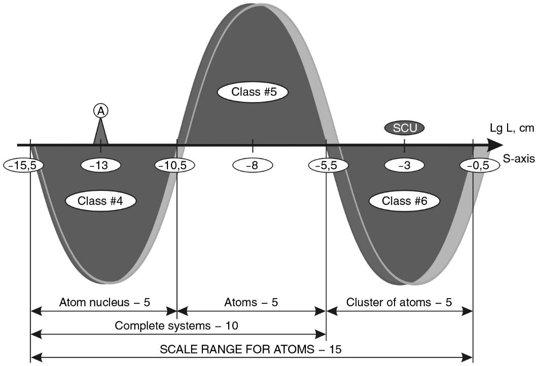 Fig. 1.17
Let us call the scale range from \(10^{14.5}\) to \(10^{28.2}\) cm the galactic scale range, which is divided into two intervals of 5 orders and one interval of 3.7 orders.
ATOMS (CLASSES #4-6). In accordance with the scheme adopted above and the position on the S-axis of the central element of the atomic class proper - the hydrogen atom - the atomic scale range should have boundaries from \(10^{-15.5}\) to \(10^{-0.5}\) cm (see Fig. 1.17) and be subdivided into three classes of 5 orders of magnitude each:
- #4. Class of atomic nuclei: \(10^{-15.5}\)- \(10^{-10.5}\) cm;
- #5. Properly atomic: \(10^{-10.5}\)- \(10^{-5.5}\) cm;
- #6. Systemically atomic: \(10^{-5.5}\)- \(10^{-0.5}\) cm.
The sizes of transient objects found in various traditional classifications should be related to our model points: \(10^{-15.5}\), \(10^{-10.5}\), and \(10^{-5.5}\) cm. Let's see if this is the case?
Let's start with CLASS #5 - the PROPERLY ATOMIC CLASS. Its center according to the model corresponds to the size \(10^{-8}\).
By the way, this size (\(10^{-8}\) cm) is so characteristic of atomic physics that it got its own name - "angstrom"
The right boundary - \(10^{-5.5}\) cm, the left boundary - \(10^{-10.5}\) cm. Recall that the most common element in the Universe is hydrogen. The diameter of a hydrogen atom is approximately 1.4 × \(10^{-8}\) cm. Several other most common chemical elements have the same atomic diameter.
The diameters of atoms of all other elements do not exceed \(10^{-7}\) cm. Atoms to the right of this size are not found in nature. The class boundary expected by the model is \(10^{-5.5}\) cm. The deviation is significant - one and a half orders of magnitude. These one and a half orders of magnitude are filled in nature with molecules of all levels of complexity: from simple to protein and high polymers.28
Let us now consider the left dimensional limit of the existence of atoms - \(10^{-10.5}\) cm. On Earth, atoms with this size can be obtained only in artificial conditions, when one of the electrons is replaced by a negative meson. Such systems are called mesoatoms29. Their diameters are very close to the transition size: for mesohydrogen - about 5 × \(10^{-11}\) cm (or \(10^{-10.5}\) cm).
"The main feature of mesohydrogen is that the radius of the meson orbit is about 200 times smaller than the Bohr radius. Therefore, the positive charge of the proton is very shielded, and mesohydrogen in many respects behaves as a neutral particle similar to the neutron."30 Here the transitive essence of mesoatoms is clearly manifested: on the one hand it is an atom, and on the other hand - a particle, as if a neutron.
In space in the region of transitional sizes (\(10^{-10.5}\) cm) there are atoms compressed in the interior of white dwarfs. Calculations show31 that the distances between atoms decrease when atoms are compressed in the interior of white dwarfs. At distances of about \(10^{-10}\) cm, the electron shells of atoms no longer exist - they are "stripped off", and the nuclei of atoms become "bare". It is at such distances between atoms that the degenerate state of gas32 described by Fermi statistics occurs.
Thus, the scale limits of the existence of atoms in their simple and molecular forms coincide with the model ones (\(10^{-10.5}\)...\(10^{-5.5}\) cm). However, if we compare the large-scale range of existence of atoms with the large-scale range of existence of stars, we find a significant difference. For stars, we have some examples of supergiants reaching the upper threshold of the model class by their sizes. For atoms, we see that their sizes do not reach the upper model threshold (\(10^{-5.5}\) cm) by more than one order of magnitude.
Thus, the transition from systems of the atom type to systems of the nuclei type takes place at the boundary of two model classes of SW - \(10^{-10.5}\) cm, and this statement does not raise any objection. The upper model boundary of the atomic class raises certain doubts.
Only the following can be stated with absolute certainty. The right model boundary (about \(10^{-5.5}\) cm) limits in nature the size of systems consisting of atoms with individual differences in composition (biomacromolecules). In these systems, the appearance or disappearance of one atom leads to a qualitative change of the whole system.
NUCLEI OF ATOMS (CLASS #4). Using the technique of determining the radii of atomic nuclei33, we can obtain a fairly accurate diameter of the nucleus of the hydrogen atom proton. It is equal to 1.62 × \(10^{-13}\) cm. In addition to the fact that "...the radius of charge distribution inside the proton is equal to 0.8 × \(10^{-13}\) cm, the radius of magnetic moment distribution in the proton and neutron were approximately the same 0.8 × \(10^{-13}\) cm."34 The diameters of the nuclei of all other atoms, determined by the simplified formula R = 1.3 × \(10^{-13}\) A1/3 cm adopted in nuclear physics, lie in the range from 2 to 15 fermi (where A is the number of nucleons in the atomic nucleus).
1 fermi = \(10^{-13}\) cm. Similarly to the angstrom (\(10^{-8}\) cm) in the structural class, the central dimension of the nuclear class, i.e., the dimension of highest stability, also has a proper name - "fermi". This once again indirectly confirms the adequacy of the SW model to the real properties of matter.
As for the lower boundary of the nuclear subclass, according to M. A. Markov35, it belongs to the size of \(10^{-15.5}\) cm, which was the boundary of penetration into the microcosm. The range of sizes from \(10^{-15.5}\) to \(10^{-13}\) cm (according to M. A. Markov) is the world of strange particles, the world of details of the neutron and proton structure.
Strange particles in particle physics are called K-mesons and hyperons.
The maximum energies currently available (we are talking about the 1980s) in the laboratory are of the order of 1000 GeV, to which correspond the minimum distances of about \(10^{-17}\) cm36. The author provides that if experimental physics manages to penetrate into the depth of matter at least to \(10^{-18...20}\) cm, it will come in close contact with the internal structure of electrons. To the right of the center point (-13) of this CLASS #4 are all the nuclei whose maximum size is close to \(10^{-12}\) cm. So, CLASS #4 in the SW model corresponds to the features of the traditional systematization of the particle world. Its model center coincides with an important for physics size - "fermi." Here also "dwells" the most stable particle of our world - the proton. To the left 2.5 orders of magnitude from the center is the world of strange particles. One order of magnitude to the right of the center is the nuclei of atoms.
It should only be noted that in the size range from 1.5 × \(10^{-12}\) cm to \(10^{-10.5}\) cm on the S-axis there is essentially an empty space, not filled with any natural formations and systems that would be well known to science. This is so strange, because nature does not tolerate emptiness, that there are two assumptions: either in this range is really very low stability of systems, or science has yet to discover a whole range of systems "missed" by it with these dimensions. Purely speculatively, one can PROPOSE that there may exist some giant nuclei or their complex nuclear clusters reaching sizes of \(10^{-10}\) cm. In addition, by analogy with the stellar scale range, one can PROPOSE that in this size range there exist size-limited "clusters" of electrons. After all, there are globular and scattered clusters of stars in a similar place in SWS.
Strange as it may seem, the least we can say about the system-atomic class, which presumably occupies 5 orders of magnitude from \(10^{-5.5}\) to \(10^{-0.5}\) cm (CLASS #6). By analogy with stars, we can PROPOSE that we are talking about some atomic clusters united by electromagnetic interactions, and the sizes of these clusters cannot exceed 5-10 mm.
Thus, we can confidently assert that the atomic scale range occupies at least 10 orders on the S-axis, which are subdivided into two classes of 5 orders each. Whether there is an additional third CLASS (No. 6) for the atomic scale range remains an open question.
Concluding this section, we have an opportunity to present the above-mentioned periodic classification of all systems of the Universe, which is based on the SWS model, but in a slightly different form (see Fig. 1.18).
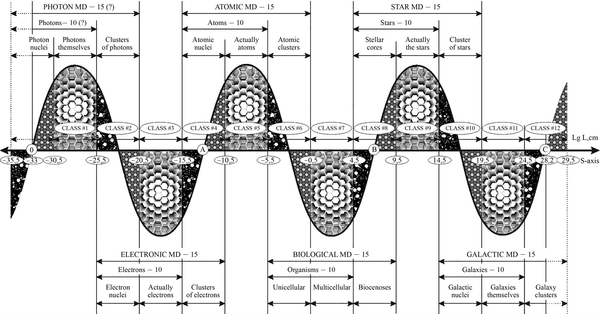 Fig. 1.18. General scale-classification scheme of the Universe objects. To create the best mnemonic image (as suggested by the editor), the sixth harmonic of scale fluctuations was used (see Section 2.5.1). The scaling length of each class is equal to five orders of magnitude. It can be seen that objects of different levels of the Universe can be present in the same scale class. For example, star clusters and galaxy nuclei are present in the same scale class #10, and electron clusters and atomic nuclei are present in the same scale class #4. We see that all 6 scale ranges (MDs) overlap each other, forming a giant scale chain of systems. Points 0, A, B, C are the points of division of the whole M-band into 3 main S-intervals, 20 orders of magnitude each: 0-A - Micro-interval, A-B - Macro-interval, B-C-Mega-interval. Different types of classes: nuclear class; structural class; system class.
Although our classification contains quite a few questions from the microworld dimensions and some relatively controversial boundaries; in general, it does not raise doubts. Since the errors and deviations are quite permissible with such a wide coverage of empirical material, and are not superimposed on each other, but mutually compensated, which leads to the preservation of a uniform periodicity throughout the S-axis. For completeness of the picture we will try here to fill the "holes" in the microworld region and to build in there two more HYPOTHETICAL scale ranges.
SUB-ELEMENTARY PARTICLES (CLASSES # 1-3). Moving along the S-axis to the region of even smaller sizes, we get into the world of structures never experimentally investigated by science. On this way we find a whole class of possible systems, about which we can only say the following.
The structural ridge closest to the atomic ridge has a coordinate of \(10^{-18}\) cm. We believe that it is "populated" by electrons. Most likely, it is in this size range that the structure of the electron can be detected in time. For "the question of the radius of the most "ancient" elementary particle - the electron - is still a mystery. Up to the smallest distances available with modern experimental techniques (\(10^{-15}\) cm), the electron behaves as a point particle."37
This was written in 1972, and since then physicists have been able to penetrate 2 more orders of magnitude into the microcosm, but the structure of the electron still appears to be point-like.
On the basis of the SW model, its size may be of the order of \(10^{-18}\) cm with a nuclear core of \(10^{-23}\) cm (see Fig. 1.19). Then, by analogy with the previously identified S-Ranges, we can predict the existence of an Electron Scale Range with a length of 15 orders of magnitude. An even lighter, almost weightless particle-wave is the photon. According to the logic of the model, it has the only free place on the last, extremely left ridge of the SWS - \(10^{-23}\) cm.
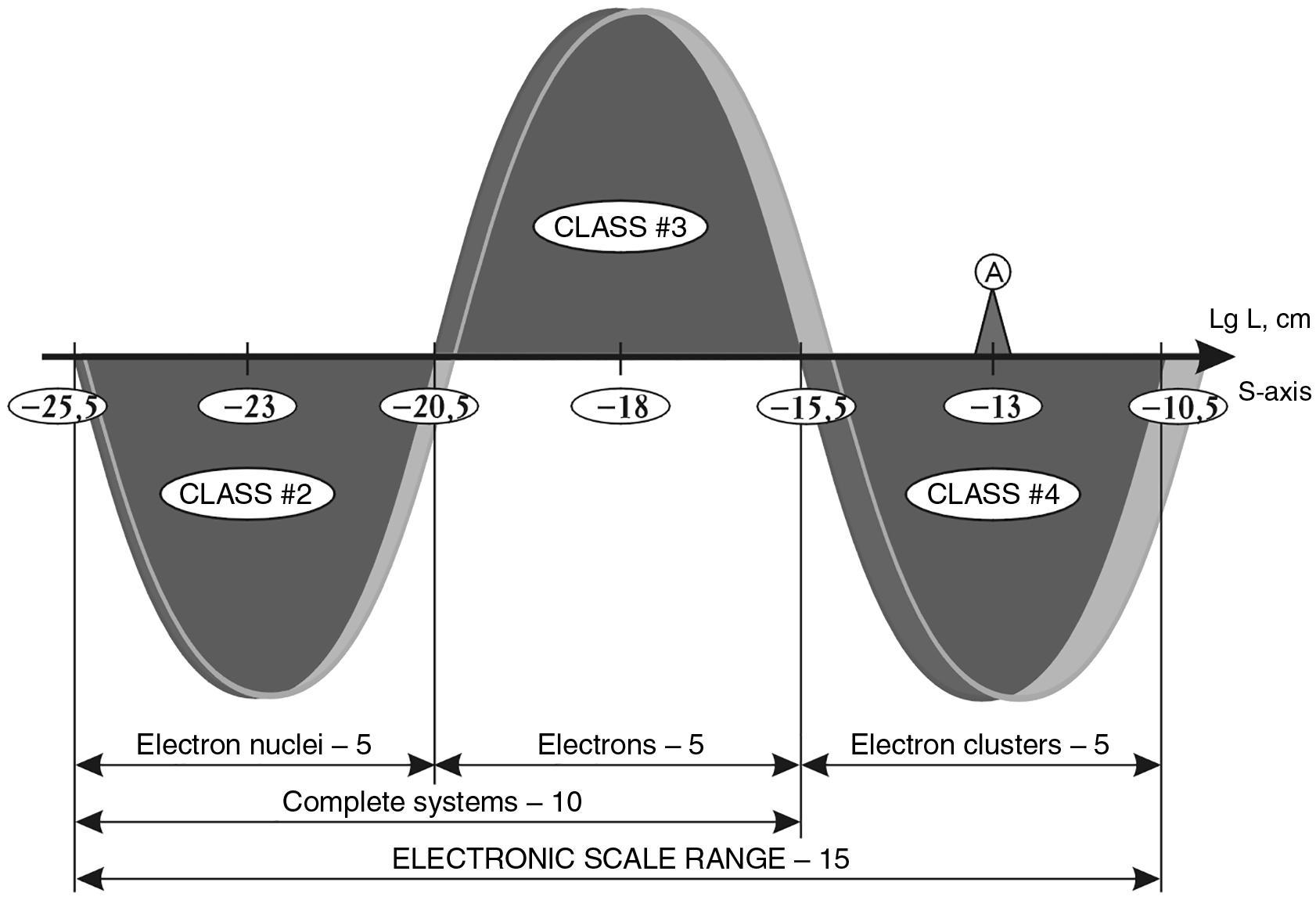 Fig. 1.19
We should not be confused by the fact that the photon, as well as the electron, has a wave structure. We are talking about the size of its corpuscular essence. Then we can PROPOSE that there is a truncated photon scale range from \(10^{-33}\) cm to \(10^{-20.5}\) cm, with the hypothetical maximon acting as the photon nucleus.
However, it should be noted that both photon and electron can be not so much particles with clear boundaries as vortices or excitations (like solitons) in the ether and, therefore, their sizes are still an open question requiring deep theoretical and experimental study. Moreover, the conducted theoretical investigations of this question in the work of N. P. Tretyakov and S. P. Tretyakov and S. I. Sukhonos ("Arithmetic of the Universe" in the book "Man on the Scale of the Universe", Moscow: New Center, 2004) showed that practically all elementary particles are four-dimensional resonances of the maximon medium. Proceeding from this assumption, it is rather problematic to represent them as similar bodies of macro- and mega-diameter range.
-
Willy K., Dethier V. Biology (biological processes and laws). M.: Nauka, 1979. P. 31. ↩
-
Vernadsky V. I. Biogeochemical Essays. M.-L.: ANS SSSR, 1940. P. 73. ↩
-
Kamshilov M. M. Evolution of the Biosphere. M.: Nauka, 1979. P. 60. ↩
-
Willy K., Dethier V. Biology (biological processes and laws). Moscow: Nauka, 1979. ↩
-
Allen K. W. Astrophysical Magnitudes. M.: Mir, 1977. ↩
-
Aghekyan T. A. Stars, Galaxies, Metagalaxy. M.: Nauka, 1981. P. 64. ↩
-
Aghekyan T. A. Stars, Galaxies, Metagalaxy. M.: Nauka, 1981. P. 64-72. ↩
-
Allen K. W. Astrophysical Magnitudes. M.: Mir, 1977. P. 396. ↩
-
Allen K. W. Astrophysical Magnitudes. M.: Mir, 1977. P. 320-321. ↩
-
Martynov D. Ya. Course of General Astrophysics. M.: Nauka, 1979. P. 202. ↩
-
Shklovsky I. S. Stars. Their birth and death. Moscow: Nauka, 1977. ↩
-
Shklovsky I. S. Stars. Their birth and death. Moscow: Nauka, 1977. P. 161. ↩
-
Baade W. Evolution of stars and galaxies. M.: Mir, 1966. P. 31. ↩
-
Aghekyan T. A. Stars, Galaxies, Metagalaxy. M.: Nauka, 1981. P. 402. ↩
-
Zonn W. Galaxies and quasars. M.: Mir, 1978. P. 59. ↩
-
Vorontsov-Vel'yaminov B. A. Extragalactic Astronomy. M.: Nauka, 1978. P. 222. ↩
-
Vorontsov-Vel'yaminov B. A. Extragalactic Astronomy. M.: Nauka, 1978. P. 184. ↩
-
Vorontsov-Vel'yaminov B. A. Extragalactic Astronomy. M.: Nauka, 1978. P. 184. ↩
-
Baade W. Evolution of stars and galaxies. M.: Mir, 1966. P. 208. ↩
-
Vilkovisky E. Y. Quasars. M.: Nauka, 1985. P. 122. ↩
-
Vilkovisky E. Y. Quasars. M.: Nauka, 1985. P. 146-147. ↩
-
Martynov D. Ya. Course of General Astrophysics. M.: Nauka, 1979. P. 447. ↩
-
Martynov D. Ya. Course of General Astrophysics. M.: Nauka, 1979. P. 447. ↩
-
Ginzburg V. L. Some problems of physics and astrophysics // Physics today and tomorrow. L.: Nauka, 1973. P. 43. ↩
-
Vorontsov-Vel'yaminov B. A. Extragalactic Astronomy. M.: Nauka, 1978. P. 428. ↩
-
Vilkovisky E. Y. Quasars. M.: Nauka, 1985. P. 64, 98. ↩
-
Martynov D. Ya. Course of General Astrophysics. M.: Nauka, 1979. P. 452. ↩
-
Danielson F., Alberti R. Physical Chemistry. Moscow: Higher School, 1967. P. 603. ↩
-
Goldansky V. I., Shantorovich V. P. Current state of research "new" atoms" // Physics of the XX century. Development and Prospects. M.: Nauka, 1984. P. 136-187. ↩
-
Goldansky V. I., Shantorovich V. P. Current state of research "new" atoms" // Physics of the XX century. Development and Prospects. M.: Nauka, 1984. P. 139. ↩
-
Martynov D. Ya. Course of General Astrophysics. M.: Nauka, 1979. P. 210. ↩
-
Shklovsky I. S. Stars. Their birth, life and death. Moscow: Nauka, 1977. P. 154. ↩
-
Mukhin K. N. Physics of the atomic nucleus // Experimental nuclear physics. T.1. Moscow: Atomizdat, 1974. P. 50-70. ↩
-
Y. M. Shirokov, N. Yudin. P. Nuclear Physics. Moscow: Nauka, 1972. P. 55. ↩
-
Markov M. A. On the Nature of Matter. Moscow, 1976. ↩
-
Yavorsky B. M., Detlaf A. A. Reference book on physics. Moscow: Nauka. Fizmatlit, 1996. P. 538. ↩
-
Y. M. Shirokov, N. Yudin. P. Nuclear Physics. Moscow: Nauka, 1972. P. 56. ↩