Bimodality of distribution atoms by size
In the classification discussed above, one of the most interesting parts of the S-axis is the one where atoms are located. It has two most characteristic points on the S-axis: the average size of an atom and its nucleus. According to refined calculations, the most characteristic sizes for these systems are 1.6 \(\times\) \(10^{-8}\) cm and 1.6 \(\times\) \(10^{-13}\) cm, respectively.
ATOMS (CLASS #5). Atomic radii are determined by the closeness of atomic proximity in the structure of molecules and crystals. The radius (r) obtained in this way corresponds approximately to the radius of the radial density maximum in the charge distribution of neutral atoms. In addition, the value 2r, or atom diameter, is approximately equal to the gas-kinetic diameter of motion of single-atom molecules. If we use the values of r for various atoms given in the reference book of C. W. Allen1, we can construct a histogram of the TEM distribution of chemical elements as a function of atomic diameter (see Fig. 1.50).
Analysis of the histogram shows that there are two special dimensions on the S-axis around which the values of atomic diameters are statistically concentrated.
These two special sizes, or modes,
By the way, a weakly expressed third mode can also be distinguished, but we will leave this question outside the brackets of our consideration for the time being.
have the following coordinates on the S-axis: the first mode is 1.2...1.6 \(\times\) \(10^{-8}\) cm, and the second mode is 2.4...3.6 \(\times\) \(10^{-8}\) cm.
Note that for different elements only the coefficients before \(10^{-8}\) change, so further we will specify only these coefficients for the sizes of TEM elements.
The first mode includes items such as:
- hydrogen - 1.4
- carbon - 1.5
- nitrogen - 1.4
- oxygen - 1.2
- fluorine - 1.2
To the second mode, about 60 of the remaining most common elements in nature.
Moreover, HELIUM - the second number, coming right after HYDROGEN in the Mendeleev table of elements and terms of prevalence in the Universe, has a diameter that belongs not to the first mode, which would seem to be very logical, but to the second - 2.44 \(\times\) \(10^{-8}\) cm. The tendency for the diameter of an atom to increase as its nucleus and the number of electrons in orbit increase is simple and understandable. However, a closer look reveals a very contradictory picture: this trend has a "reciprocating" character. For illustration, we have constructed the simplest diagram (see Fig. 1.51) of the dependence of the atom diameter on the group number in the periodic system of elements of D. I. Mendeleev. Analyzing this diagram, we see that as we move along the order number of the elements, the same pattern is manifested: a sharp jump in the size of the atom of group I at the beginning of each period and a subsequent slowing decrease in the size of the atom as we approach the end of the period.
If we do not take into account inert gases, it seems that the completion of shells to the maximum completeness, starting from period III and further, is possible only within a very narrow range of sizes - 2...3.6 angstroms.
Moreover, if we look carefully at the constructed diagram, we get the impression that there are two "centers of attraction" of all "trajectories", two regions of increased stability on the S-axis: the first - in the region of sizes 1.2-1.6 angstroms (I and II periods), the second - in the region of sizes 2.4-3.6 angstroms. They are highlighted on the diagram by spots.
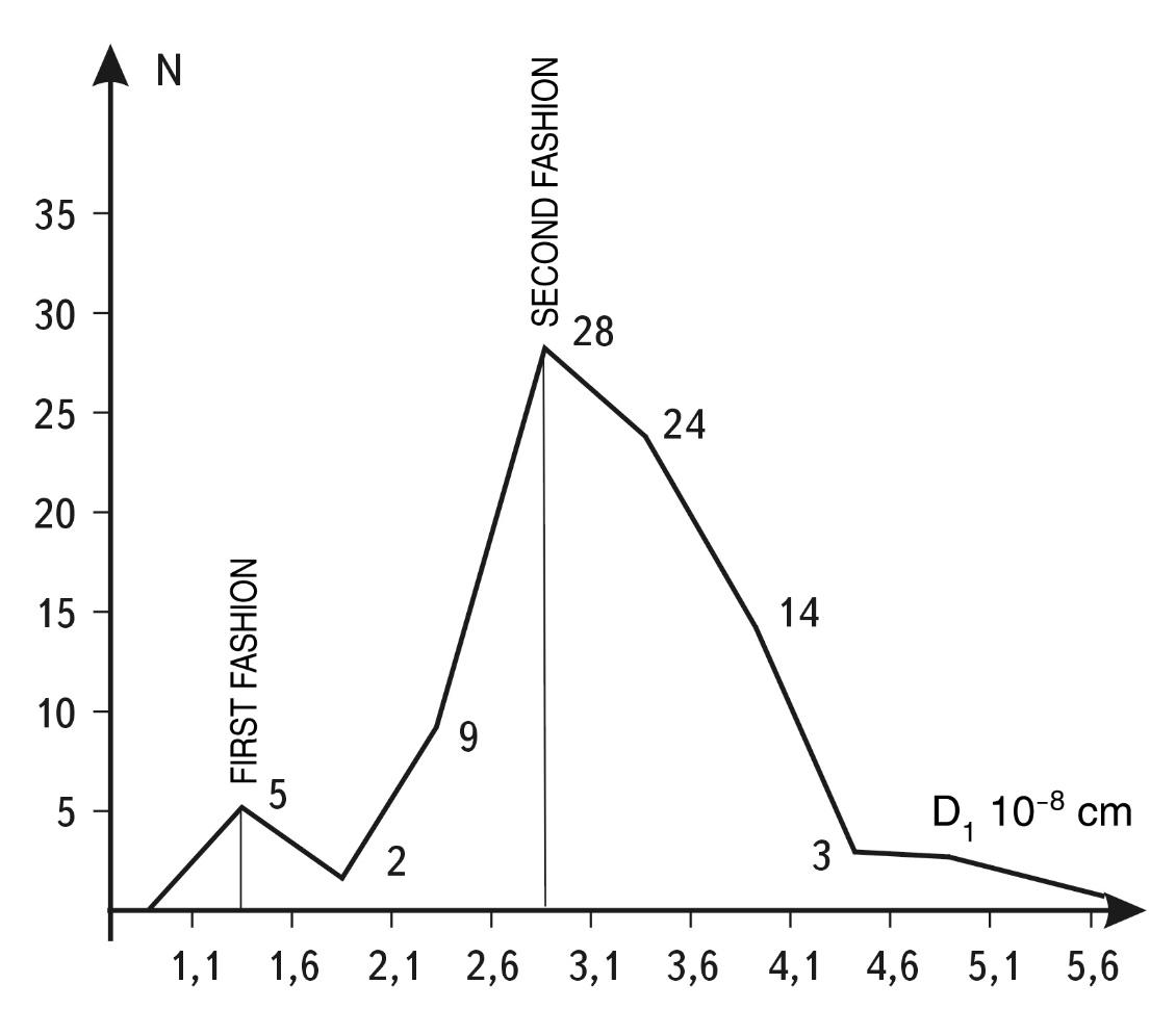 Fig. 1.50. Histogram of distribution of elements of the Mendeleev Table of Elements (TEM) depending on the diameter of elements. The histogram shows that all the diversity of the atomic composition of the Universe is associated with two main sizes (modes) - 1.4 and 2.8 angstroms. If we construct a similar histogram, taking into account the number of atoms of each element in the Universe, hydrogen would give the first mode a weight of more than 90%, and helium would give the second mode a weight of about 7%. The other elements would essentially provide an insignificant background that can be neglected. This indicates that the two modes we have distinguished are extremely representative from any point of view
Figuratively speaking, the elements of each new group formed far away from these regions are rapidly attracted by these regions as their mass grows, and the "trajectories" of each period are "bent" by the attraction of these two regions.
This unique fact can be interpreted as follows.
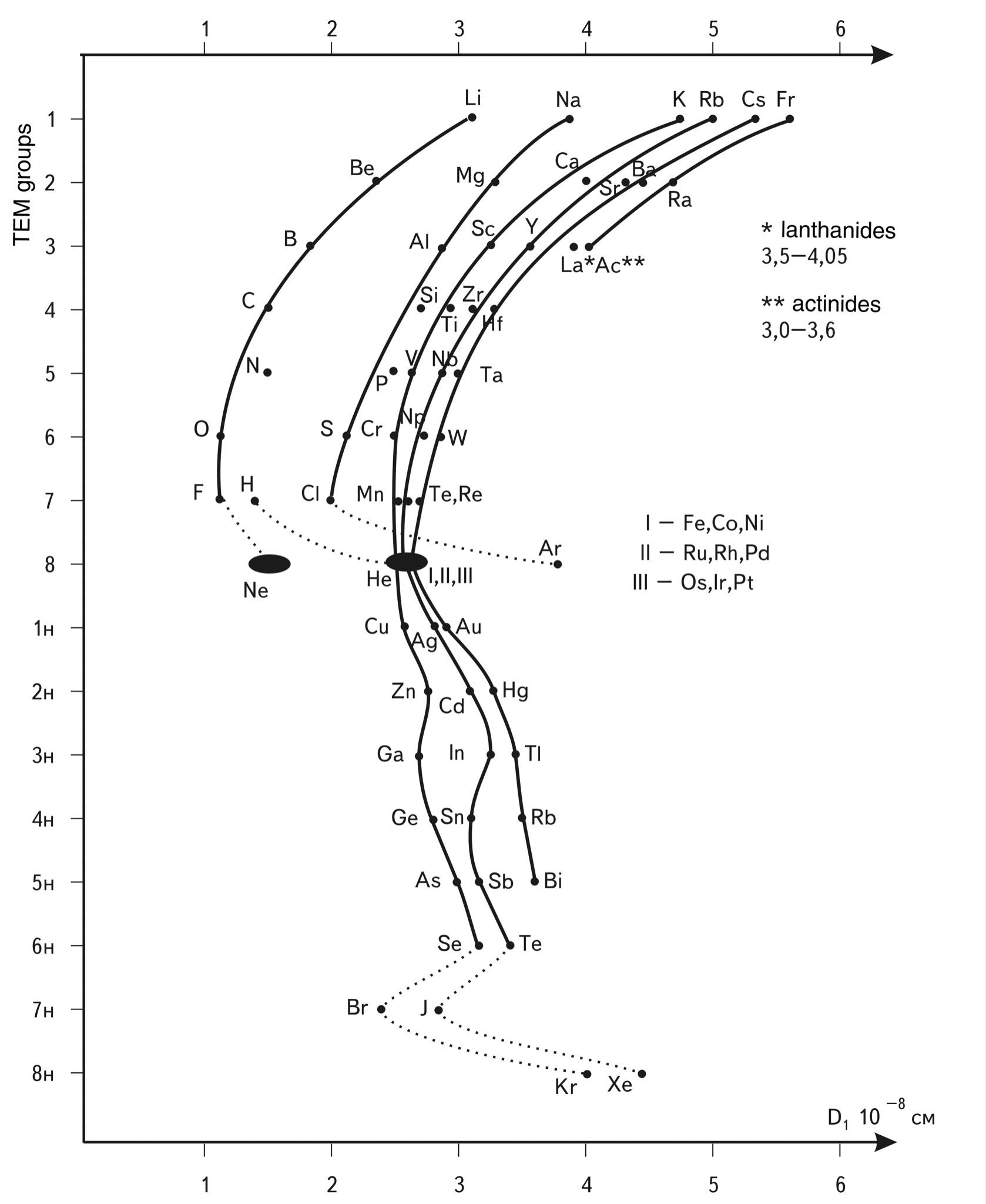 Fig. 1.51. Diagram "atom size - group number" for the Mendeleev Periodic Table of Elements of elements.
The diagram shows that the rows are built approximately "parallel" to each other. In order not to form a "mush" of points on the diagram, a separate place is allocated for the elements of the lower rows of the TEM of large periods, and the numbers of groups for the lower rows are marked with the index "n". As a result, the in-plane unfolded diagram of atom distribution along the S-axis is obtained.
The choice of such a formal criterion as group number as the second coordinate is due to the desire to emphasize the size distribution of atoms. It would be possible to construct more physically filled diagrams, taking as a second parameter, for example, the ionization potential or the electron distribution density in the volume of the atom, but the essence of this would not change much.
Analysis of the diagram shows that the size of the atoms increases as the mass of the atoms increases. This quite logical phenomenon has, however, at first sight, a very strange internal manifestation: the growth of sizes does not occur gradually but by leaps. These jumps are seemingly illogical: all elements, from which the periods begin, are the largest atoms in their periods, although they have the smallest number of protons and electrons
The stability of the configuration of electron orbits of atoms increases when they fill the SUSTAINABLE SPACE cells with two main characteristic (stable) sizes - (1.2-1.6) and (2.4-3.6) angstroms.
It should be noted that all "trajectories" in the diagram behave very similarly. The sequences on which atoms "sit" are shifted towards larger sizes, and their lower parts, populated by limit atoms, appear in a very narrow dimensional zone as if this region of the S-axis draws them into itself.
The bimodality revealed above leads to the need for some refinement of the model of SW built by us earlier. In fact, if the first mode (~1.6 \(\times\) \(10^{-8}\) cm) is calculated by this model, the significant second mode (~3 \(\times\) \(10^{-8}\) cm) is not predicted in advance by the model. If we take into account the role of atoms as the most important elements of the structure of the Universe, this reliable fact should not be neglected.
So, once again, let's record the results obtained.
First, the stable size of 1.6 \(\times\) \(10^{-8}\) cm, which gives the SW model, is represented not only by hydrogen but also by four other most abundant elements in the Universe (excluding helium), whose mass fraction (see Table 1.2) is more than 3 times larger than that of all other elements. Second, next to this most "weighty" size, we find another distinguished size that is almost 2 times larger than the first one, about 3.0 \(\times\) \(10^{-8}\) cm. This size characterizes most of the other elements of the Universe, both in terms of their number (60 TEM elements) and mass.
TSWs, only somewhere about 30 other elements have sizes not belonging to the two main stable sizes, but these 30 elements in their number in the Universe are not more than 0.01 % (see Table 1.2). In principle, at the first stage they can be not considered at all due to their extremely insignificant fraction.
Table 1.2.
Prevalence of element groups in the Universe2. For hydrogen the value of 100 is accepted
| Group of elements | Number of atoms | Weight |
|---|---|---|
| Н | 100 | 100 |
| Don't | 8,5 | 34 |
| C, N, O, Ne | 0,116 | 1,75 |
| Metals, etc. | 0,014 | 0,50 |
| Total: | 108,63 | 136,25 |
Consequently, if we consider the crest of the SWS in the atomic size region, we should be guided mainly by two sizes (taking into account a small dispersion). One size is known to us, we calculated it using the scale symmetry coefficient - \(10^5\). The other is an unexpected size for our model; its existence was not predicted by our model in its original form.
By the way, the question may arise, why do we pay so much attention to a narrow range of sizes, which occupies less than one order of magnitude on the S-axis? After all, in the Universe there exist both molecules and particles whose sizes are close to two calculated sizes.
The answer is simple. The weight fraction of molecules and dust in the Universe in relation to free atoms is vanishingly small, as well as the weight fraction of planets and comets. If we mentally start moving along the S-axis to the right of the two sizes we have selected, then practically up to the sizes of stars, which is 20 orders of magnitude to the right along the S-axis, we cannot find objects in the Universe, the mass fraction of which would give us at least some elevation on the diagram on the background of the mass fraction of atoms.
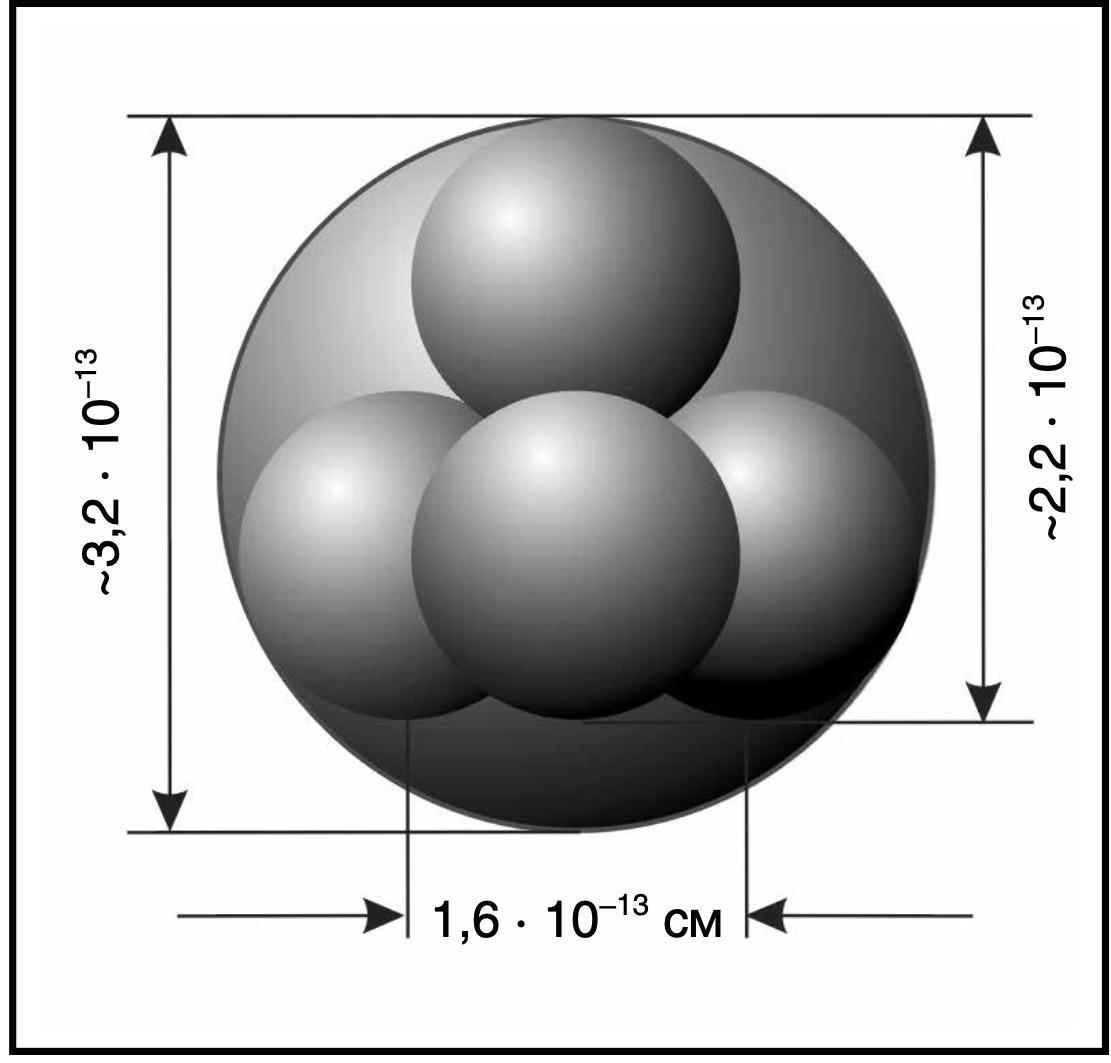 Fig. 1.52. The helium nucleus, or α-particle, consists of two neutrons and two protons
If we move from the atomic ridge to the left, then after five orders of magnitude we will find ourselves in the scale zone of atomic nuclei (CLASS #4). These contain more than 99.9% of the atomic mass. For them, too, it is important to study the characteristic points on the S-axis.
ATOMIC NUCLEI (CLASS #4). Let us consider how the nuclei of atoms are distributed by size. The radii of light nuclei are determined3 by the empirically derived formula R=1.3 \(\times\) \(10^{-13}\) \(\times\) A\(^{1/3}\) cm.
In this case, we are interested in two nuclei - hydrogen and helium.
As mentioned in Section 1.3.2, the diameter of a Hydrogen Nucleus consisting of a single nucleon is 1.6 \(\times\) \(10^{-13}\) cm4.
The diameter of the helium nucleus, which also has extremely high stability and consists of four nucleons, is at least twice that of the hydrogen nucleus, 3.2 \(\times\) \(10^{-13}\) cm (see Fig. 1.51).
Since hydrogen and helium in general occupy more than 90% of the matter in the Universe, we can talk about bimodality in the distribution of atomic nuclei.
However, both for atoms and their nuclei, we can distinguish a third mode in the distribution, which is occupied by the nuclei of the elements of the iron group. For the iron nucleus (A = 56) we obtain a size of 10.7 \(\times\) \(10^{-13}\) cm.
One mode is for the proton, i.e., the hydrogen nucleus, is 1.6 \(\times\) \(10^{-13}\) cm (73% of the entire visible mass of the Universe). The other mode for the helium nucleus is 3.2 \(\times\) \(10^{-13}\) cm (25% of the entire visible mass of the Universe).
It should be noted that, unlike atoms, the distribution of nuclei by their sizes is continuous. The nuclei on the S-axis are not concentrated into two groups if their distribution is considered without taking into account the mass fraction. So, we see the obvious fact of the bimodal distribution of the main elements of the Universe on the S-axis in their nuclear and atomic forms.