Star Waves
If atoms are the basic elements of the Universe, then stars are the basic objects in which they are concentrated. Therefore, analyzing the regularities of the distribution of stars by their sizes is as important for us as analyzing the distribution by the sizes of atoms.
Unfortunately, in the most accessible reference books we could not find any tabular data on the statistics of the distribution of all types of stars by their sizes, similar to the distribution of atoms. We had to resort to an indirect, roundabout way, partly calculating their sizes by known astrophysical formulas.
The main CHALLENGE was that if the coordinate of the upper point of the SWS ridge (CLASS #9), corresponding to a size of \(10^{12}\) cm, is special for stars, then this coordinate point should show itself in the dependencies of the most important parameters of stars on their sizes.
Before proceeding to this elucidation, it is necessary to make some general remarks on the CHARACTER OF STAR EVOLUTION in the Metagalaxy.
Astrophysicists, analyzing the chemical composition of stars and the distribution of stars in different parts of our Galaxy, have found over time that stars can be fairly reliably divided into two types. "Although the chemical composition of most stars is almost identical, they do have slight differences. These do not affect the luminosity or color of the star very much but can be detected in the spectra. Almost all stars are composed mainly of hydrogen and helium: for example, most stars in our region of the Galaxy have only 1% of their mass made up of heavy elements, and very few stars have even smaller proportions of heavy elements, as low as 0.01%. Stars like the Sun are called stars rich in heavy elements; in our Galaxy, these stars belong to population I, while stars poor in heavy elements belong to population II1.
According to the famous astronomer V. Baade2, this division into two groups is not accidental but is associated with two epochs of star formation.
The first epoch of star formation took place simultaneously not only in the Local Group of galaxies but also everywhere in the Metagalaxy. It refers to the moment of the Metagalactic expansion (\(t_0 \sim 10^9\) years), when there was a rapid burst of star formation from the primary hydrogen-helium ball, apparently in the already formed protogalactic clouds. This was the very first generation of stars.
At present, due to the high lifetime of the first generation of stars, we have the opportunity to observe these patriarchs in the sky, although their number has noticeably thinned. It is these first-born stars of the Universe that are called type II stars because of the peculiarities of their distribution in our Galaxy – they are mainly located in spherical halos of galaxies and very often in globular clusters of halos (see Fig. 1.53).
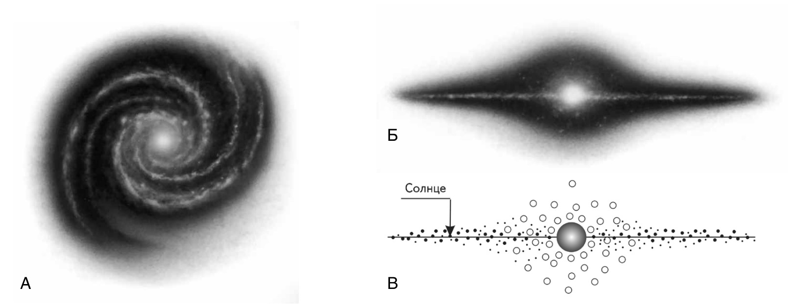 Fig. 1.53. View of our Galaxy from above (A) and from the side (B). In the center is a spherical halo, which includes stars of population type II (white circles in diagram C – the first generation of stars) and spiral arms consisting of stars of population type I (black dots – the second generation)
It is believed that the first epoch of star formation was followed by a second, longer epoch, during which stars of the galactic disk were formed in our Galaxy.
The second epoch, according to V. Baade, was less turbulent and probably lasted several billion years.
Now, according to S. A. Kaplan3, the third epoch is underway, which should cease in the Galaxy in \(10^8\)–\(10^9\) years, since at the present rate of star formation the reserves of the interstellar medium will not be sufficient for a longer time.
At present, sufficient observational data have been accumulated to show that the star formation process is not uniform. Epochs of rapid star formation are separated by periods of relative quiescence.
For our purposes, however, it is important to note that the very first stars began to appear at the time of the expansion of the Metagalaxy, when its size was about \(10^{27}\) cm (1 billion years).
It is obvious that the primary stars could consist only of hydrogen and helium, since the appearance of heavier elements, according to the generally accepted concept of the chemical evolution of matter in the Universe, could occur already during the evolution of the stars themselves.
Other stars, which are mainly concentrated not in the halo but in the Galaxy disk, appeared at the next stage. They differ significantly from the first stars by their location in the Galaxy itself, by their saturation with heavy elements, and by other parameters. These two types of stars are easily distinguished in astrophysics as two relatively independent classes. In the following, we will show this in more detail.
Now let us consider the peculiarities of interdependence of physical parameters of stars. Modern astronomy has methods for determining the main stellar characteristics: luminosity, surface temperature (color), radius, chemical composition, and mass.
An important question arises: are these characteristics independent? It turns out that they are not.
First of all, there is a functional dependence connecting the radius of a star, its bolometric (integral over the entire spectrum) luminosity and surface temperature. In addition, as early as at the beginning of our century, the Dane Hertzsprung and the American Ressel established the dependence between the luminosity of stars and their color on a large statistical material. A remarkable feature of the latter dependence was that the position of all the stars of the Universe on the diagram "Luminosity – spectral class, or color" (the Hertzsprung-Ressel diagram) turned out to be by no means disorderly or random (see Fig. 1.53A). The stars form certain sequences (see Fig. 1.53B), among which there is the most rich in stars – the GENERAL STAR LABEL (GS).
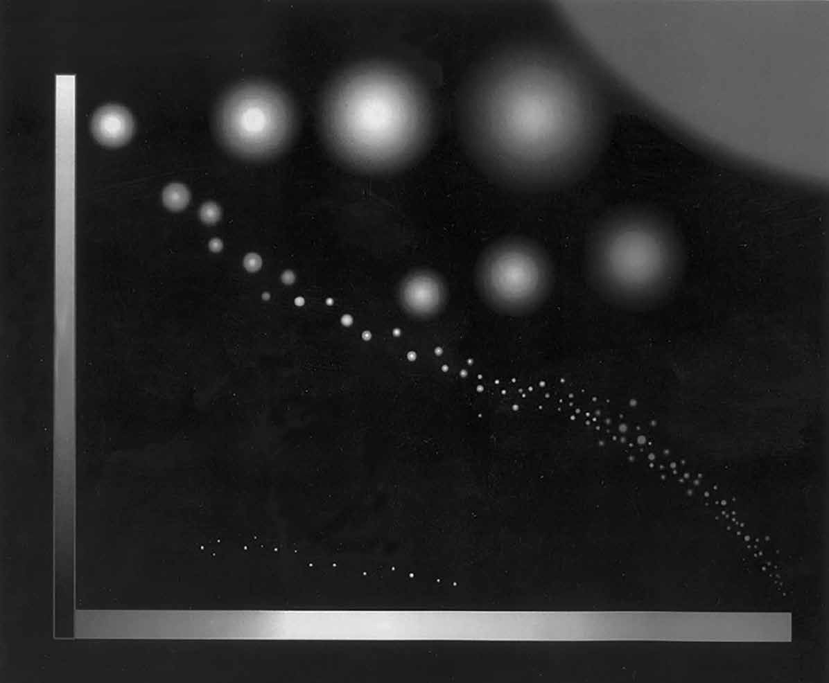 Fig. 1.54. Location of the stars of the Universe on the diagram "Absolute stellar magnitude – spectral class (color)", which was discovered by Hertzsprung and Ressel
The star densification zones in diagrams of this type are often called branches and are depicted as lines along which the evolution of stars takes place.
The fact that practically all stars "choose" very narrow parametric zones in diagrams of this type testifies to the presence in the nature of stars (and hence in the bulk of matter) of stable parameter ratios that ensure their stable and long existence. Although the presence of such stable selected parameter zones is an interesting problem in itself, what is of interest to us are primarily the special sizes in this range of scales. Therefore, using the values of these parameters, let us calculate the sizes and construct similar diagrams for stars, but in slightly different coordinates. For this purpose, it will be convenient to construct the "spectral class - diameter" diagram (Sp-D), on which the interposition of the sequences of stars is rather accurately preserved. Typical sizes of population type I stars are taken from the reference*. For type II population stars, the sizes were determined from a known relation: \[ M_b = 42.31 - 5 \lg \left( \frac{R}{R_0} \right) - 10\ T_{\text{eff}}, \tag{1.9} \]
Where:
- \(M_b\) is the absolute bolometric stellar magnitude
- \(T_{\text{eff}}\) is the effective temperature of the star
- \(R\) is the radius of the star
- \(R_0\) is the radius of the Sun
The relation (1.9) can be rewritten for the diameter (\(D\)) of the star:
\[ \lg D = 19.62 - 0.2M_b - 2 \lg T_{\text{eff}} \tag{1.10} \]
The values of \(M_v\) and \(T_{\text{eff}}\) were taken from the reference book (See: Allen K. W. Astrophysical Magnitudes. M.: Mir, 1977) and after conversion by the formula:
\[ M_b = M_v + BC, \tag{1.11} \]
where:
- \(M_v\) is the absolute visual stellar magnitude
- \(BC\) is the bolometric correction
The dimensions for the population type II stars were obtained using formula (1.10).
All these data and calculation results are summarized in their final form in our Spectral Class–Diameter diagram (Sp–D). For convenience of comparison with other S-axis diagrams, this diagram is arranged not traditionally, but such that the dimension axis is horizontal (see Fig. 1.54).
Let us consider this somewhat unusual astrophysics diagram. Three bell-shaped functional dependencies are highlighted on it.
We emphasize once again that this diagram is unusual only in the choice and orientation of the coordinate axes, and the data for it do not differ from the data of the classical G-P diagram.
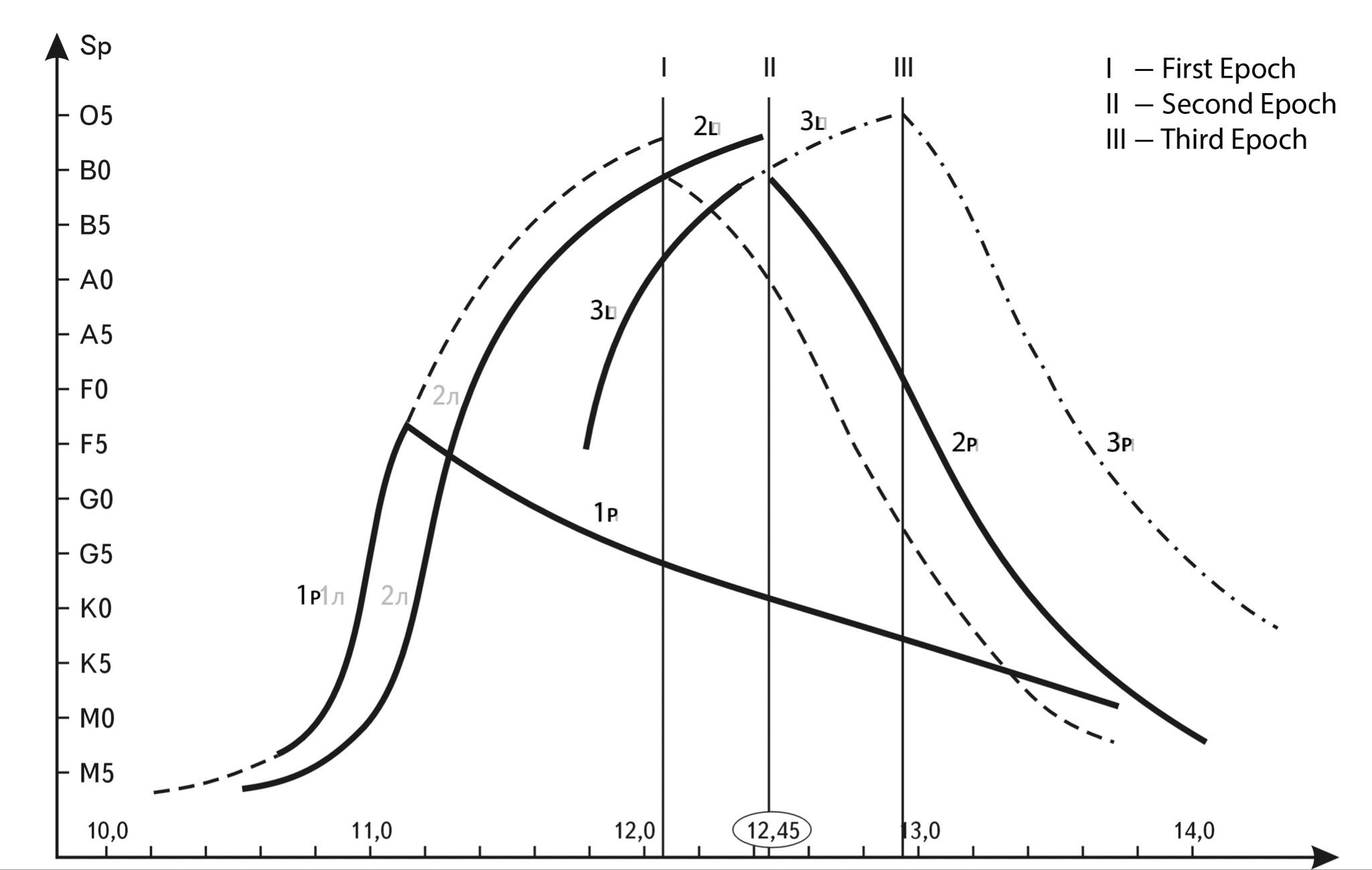
Fig. 1.55. Spectral class-diameter diagram, which was obtained by the author from the Hertzsprung-Ressel diagram by translating absolute stellar magnitude into stellar diameter. Thick lines - existing stellar sequences. Dashed lines - assumed sequences in the past (- - - ) and future (- . - . - . -)
Later we will explain why some of them are represented by dashed lines.
The average bell-shaped dependence consists of two branches: the "main sequence" - 2l (left) and the "supergiant branch" - 2p (right).
They are almost mirror symmetrical about a vertical axis that passes through the top of the bell and has a coordinate on the dimension axis equal to about 12.45.
Let us turn once again to the astrophysical ideas about stars. Recently, a consistent theory of stellar evolution has been created, in the framework of which each star describes different tracks on the Hertzsprung-Ressel diagram during its evolution (depending on the initial mass).
If the GENERAL LETTER (depicted by the line 2l in Fig. 1.55) is the main region of existence of most stars, then the supergiant branch (2p) is the subsequent stage of development of massive O and B class stars 4.
In this case, we can say that the branch of supergiants is the track of their development: due to their large mass, supergiants pass extremely quickly to the right, ending their journey at the bottom. They seem to "roll down from the top of the bell" to the right, expanding in size.
One of the peculiarities of the GENERAL sequence is that, on closer examination, it consists of parallel lines-sequences, each of which is populated by stars with a strictly fixed percentage of heavy elements (see Fig. 1.56).
The lower edge of the HEAT band is populated by stars with insignificant presence of heavy elements in the stars (the number of elements heavier than hydrogen Z = 0.01).
As one moves upward, the fraction of heavy elements increases, and at the right edge of the DIRECTIONAL FIGURE Z = 0.6.
Taking into account the fact that later stars are born in an environment richer in heavy elements, we can conclude that later stars are located higher (see Fig. 1.55) or to the right (see Fig. 1.54) than earlier ones.
Therefore, it can be stated that the main sequence is gradually "drifting" to the right, toward larger sizes (see Fig. 1.54). This allows us to take a new look at the branch of subdwarfs (1l) and the branch of red giants (1p) and make a number of PROPOSALS. Since the subdwarfs are very old stars, extremely poor in heavy elements, and their branch is noticeably shifted to the left of the main sequence branch and goes to its middle parallel to it, the following, not so groundless, assumption arises. The branch of subdwarfs is simply a remnant of the "primary main sequence", as it was at the time of the Metagalactic expansion 1 billion years ago.
It was at this moment that the first burst of star formation occurred. This is convincingly confirmed by the studies of V. Baade: "The facts indicate that before the modern epoch of star formation, there was another epoch characterized by almost simultaneous appearance or formation of stars in galaxies "5.
The branch of red giants is, apparently, the right slope of the "primary main sequence". Along it the stars of the first epoch of formation from the middle of the former GP complete their way.
All the hotter and brighter stars of the primary GP have completed their existence in a decade and a half. They simply disappeared from the diagram.
The author believes that if the primary charts could be restored, they would likely take the form of the same bell, but located to the left of the current one.
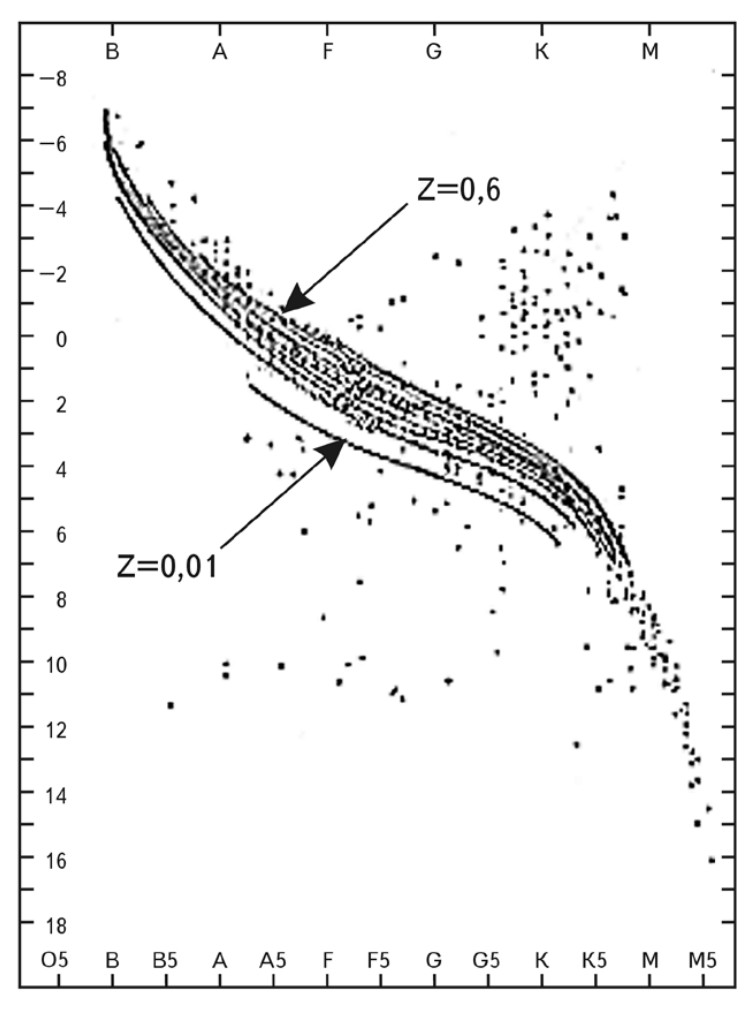 Fig. 1.56. This diagram clearly shows the "drift" of the GENERAL FOLLOW-up (GF) in the side of more brightness (and size) upwards as the transition from older stars (low heavy metal content) to newer stars proceeds
A simple geometrical restoration based on the principle of symmetry and similarity allows us to reconstruct the primary bell (dashed line), which we believe reflects the kind of diagram (I) that could be constructed immediately after the first epoch of star formation. The top of this bell would have an S-axis coordinate slightly larger than 12.0.
This idea of two domes, each of which belongs to a different epoch, agrees very well with the conclusion of V. Baade: "It would be interesting to find out whether we are really dealing with the superposition of two luminosity functions, which would mean the superposition of two mass spectra "6.
There is little left of this primary wave by now, it has settled and fallen off. In the same way, the present "bell" (II) is gradually "crumbling" with stars. Sooner or later it will lose its hot and bright top and settle down below.
If astrophysicists had lived during all 15 billion years together with stars and plotted the diagrams, they would have observed an elegant picture of rising and falling waves on the diagram (Sp -D). The wave would not just rise and fall but would follow the expanding Metagalaxy to the right.
By the way, purely visually it is very similar to an ocean wave. On the crest of this wave, the brightest and hottest stars shine to us, whose life, alas, is the shortest. True, it is necessary to note a fundamental difference in the images. Stellar waves have a discrete character, between the wave of the first epoch and the wave of the second epoch there is a gap of several billion years, so there is an empty parametric space between the branches of the diagram.
Let us summarize some results. Relying solely on a huge array of data on the parameters of many stars in the Universe, we have obtained a half-wave on the S-axis, the left edge of which (2l) rests on white dwarfs, and the right edge (2p) — on red giants inflated at the last stage of their existence. The center of this half-wave is the top of the bell-shaped dependence of the spectral class on the diameter of stars. Its modern coordinates are close to the value \(10^{12.45}\) cm.
If we accept a quite reasonable reconstruction, we can restore next to today's half-wave the wave (1l–1p) that appeared in the first billion years of the Metagalactic expansion. When the size of the Metagalaxy was close to \(10^{27}\) cm, the top of the bell corresponded almost exactly to the coordinate — \(10^{12}\) cm on the S-axis.
We can speak at least about the BIMODAL DISTRIBUTION OF PARAMETRIC FUNCTIONS OF STARS.
And the first mode is associated with the simplest first-generation stars, or as astrophysicists call them - population type II stars - they consist primarily of hydrogen.
The second mode consists of second-generation stars, or type I population stars, saturated with heavy elements to a much greater extent.
TSWs, the analysis of the distribution functions of stars by their parameters has shown that stars can be divided into two types with sufficiently high reliability.
One type of stars, which appeared mainly in the first billions of years of the Metagalactic expansion, has smaller masses and almost no heavy elements in the composition of stars. In our Galaxy, such stars form its skeleton, the halo. The second type of stars, which appeared a few billion years later (their average age is about 5 billion years), are mostly located in the flat disk of the Galaxy.
-
Hodge P. Galaxies. M.: Nauka, 1992. С. 45. ↩
-
Baade W. Evolution of stars and galaxies. M.: Mir, 1966. ↩
-
Kaplan S. A. Interstellar medium and the origin of stars. M: Nauka, 1977. С. 60. ↩
-
Efremov Yu. N. Origin and Evolution of Galaxies and Stars. M.: Mir, 1976. С. 375. ↩
-
Baade W. Evolution of stars and galaxies. M.: Mir, 1966. С. 252. ↩
-
Baade W. Evolution of stars and galaxies. M.: Mir, 1966. С. 298. ↩