Two S-waves of stability

Long-term reflections have led the author to the conclusion that characteristic (stable) sizes of the Universe cannot be explained on the basis of local interactions only. Many important sizes are determined by the boundary conditions of the scale range of the Universe. A possible physical interpretation of this conclusion will be given in the following sections, and here we will limit ourselves to its analysis within the framework of symmetry categories. Let us emphasize at the first stage the two most important dimensionless coefficients of the S-axis: \(10^5\) and \(10^{61}\).

The first coefficient is a phenomenological given, reliably manifested in the relationships of many different parameters on all scale floors. It is related to other Big Numbers, being the smallest common multiple for them: \(10^{10}\), \(10^{15}\), \(10^{20}\), \(10^{40}\). Let us call it the S - Symmetry Coefficient - SSC.

Its origin is considered in the work of the author together with N. P. Tretyakov "Arithmetic of the Universe".

There are good reasons to believe that \(10^5\) is a previously unknown to science dimensionless constant of our world, no less important than the speed of light or the mass of a proton.

The second coefficient is the most reliably determined S - INTERVAL OF THE UNIVERSE (SIU), containing 61 orders on the scale of decimal logarithms: 28 - (-33) = 61.

Its more precise value depends on the true size (diameter) of the Universe, which is estimated in the range from (3.2...6.4) \(\cdot\) \(10^{28}\) cm, which gives a spread of 61.2...61.6. Rounding here its value to the minimum value of 61, we do not pretend to the final accuracy of the calculation, for it will be possible only when we obtain reliable data on the size of the Universe and on the rate of the interaction that determines the formation of the scale-hierarchical structure of the Universe.

Comparing two dimensionless quantities 5 and 61, we see that there is no integer relationship between them. If we postpone the MS basis coefficient starting from the left edge of the S-axis, it does not fit an integer number of times into the scaling interval of the Universe, with a residual of one order of magnitude.

However, if the Universe had dimensions of 1.6 \(\cdot\) \(10^{27}\) cm, then the total length of the S-interval of the Universe would be equal to 60 orders of magnitude, which is divisible by 5 orders of magnitude 12 times without remainder. It is very important to emphasize that such a situation in the model of the expanding Universe is quite physically real, it could have arisen at the moment of expansion when the Universe had an age of about one billion years. As astrophysicists are convinced, it was at that moment (at the moment of S-SYMMETRY) that a rapid process of structure formation took place on all floors of the Universe. We have shown above that all structures formed in this process have average sizes that are surprisingly precisely 5 orders of magnitude apart along the S-axis (nucleons, hydrogen,... old stars and elliptical galaxies).

In total, these main types of systems should have been formed in the Universe according to the SWS model - twelve, not counting the primary one - maximon, closing the S-band of the Universe from the left edge and taken by us as point zero.

Of course, at present we can confidently match the 13 nodes on the S-axis with only 6-8 real types of physical systems. However, the fact that in spite of gaps in the sequence, the sizes of the main representatives of the TWENTY-THREE CLASSES on the S-axis are obtained by translation of the base coefficient \(10^{5}\) quite accurately (sometimes - phenomenally accurately), allows us to put forward the following SCENARIO OF EVENTS DEVELOPMENT OF EVENTS IN THE UNIVERSE.

At the age of the Universe of one billion years, two parameters (\(10^{5}\) and \(10^{60}\)) created a special SCALE - RESONANCE situation (S-Resonance), which had no analogs in the subsequent expansion process. Probably, that is why on the S-axis the basic structural sizes of the main classes of the Universe objects are several orders of magnitude apart with the accuracy of the coefficient 1.6 in front of their values.

Further expansion of the Metagalaxy during the last 16 billion years led to the lengthening of the scale interval by only one order of magnitude. But this was sufficient for the mismatch of the large-scale resonance.

The number and nature of the main classes on the S-axis have not changed during this time: galaxies, stars, atoms and other objects have existed at least since the age of the Universe at 1 billion years. Since then, at least one new large-scale class of systems that occupies a strictly dedicated scale interval has not yet appeared. Consequently, the NUMBER OF CLASSES EQUAL to 12 is a of S-Axis Dimensionless Constant - (SADC)(we can accept another equivalent constant - 6 waves, which form 12 half-waves, taken by us as the basis for the separation of S-classes).

Note that the number 6 was not chosen by chance. The point is that 6 is the first complex even-even harmonic in the series of integers: 1, 2, 3, 4, 5... Because 1-2-3 = 6.

So, there are currently TWO MASSIVE INVARIANTS that have remained unchanged in the expanding Universe for at least the last approximately 10 billion years. The first is 5 orders of magnitude. The second is 12 classes, or half-waves.

The partitioning of the S-axis by these two invariants occurs according to different principles, - and this is fundamental for further considerations.

The first BASIS coefficient - \(10^{5}\) - as the whole phenomenology shows, is strictly exactly deferred from the left edge of the S - Interval (from point 0), breaking the whole S-axis into essential nodes alternating after 5 orders of magnitude.

The second coefficient splits the whole S - Interval of the Universe (SIU) exactly into 12 segments irrespective of its changing length. Naturally, at different moments of the Metagalactic expansion, the division of its S-interval into 12 parts leads to obtaining segments of different lengths. If we divide its present-day length of 61 orders of magnitude into 12 classes, we get a new dimensionless value of \(10^{5.083}\), which is not a constant but grows with the expansion of the Metagalaxy. Let us call it the S-Symmetry Evolutionary Coefficient (SSEC)

It would seem that obtaining a small correction after the decimal point at such scales is an insignificant trifle. However, thanks to this correction we can make one more fundamental step, namely, to pass from a simple partitioning to a wave partitioning. After all, from the formal point of view, the division of the changing interval into constant integer 6 waves (or 12 half-waves) is nothing else than a MODEL of a MASTER WAVE, whose length depends on the right changing scale boundary of the Metagalaxy.

In this case, it turns out that the S - Wave of stability has its "shadow" - the phase-shifted EVOLUTIONAL WAVE of stability (EWS), which fits into the scale range of the Universe an integer number of times (Fig. 1.57), being a large-scale standing wave.

Recall that, according to the theory of oscillations, any standing wave always fits within the boundaries of the medium in which it propagates an integer number of times.

The characteristic stable points on the S-axis for the Evolutionary Wave depend on the radius of the Universe.

As the Universe expands, the second sinusoid, unlike the first one, will stretch to the right like an accordion, and all stable points that it sets will shift to the right along the S-axis. This allows us to make the following important PROPOSITION. In the Universe, all characteristic, stable dimensions have a BIMODAL (most pronounced) distribution. The first modes are formed by translation (shift by 5 orders of magnitude) along the S-axis from the left extreme point (10-32.8 cm) of the coefficient \(10^{5}\). All characteristic sizes of the main types of systems are associated with them.

These dimensions (with a correction factor of 1.6) are shown in the Wave of stability graph we used in the previous sections.

The second mode in the distribution of objects by their size will always be located to the right of the first mode.

As shown by calculations, these modes are formed by translation along the S-axis of the MS Evolutionary Coefficient, which is currently equal to 5.083.

Consequently, a more complete model of the Stability Wave will look bifurcated, as depicted in Fig. 1.56. The SWS has its twin - a wave with some phase shift. If you examine the figure, you can see that the crests and troughs of the second wave (EWS) - as you move from point 0 - move away from the crests and troughs of the first wave EVOLUTIONAL WAVE of stability -EWS). At the rightmost point C, the TEW is in a state of maximum stability. So, we BELIEVE that if the first wave - SWS is formed due to the integrity of the initial coefficient \(10^{5}\), then the second wave - EWS owes its origin to the integrity of waves that fit into the scale interval exactly 6 times. In both cases, the integrity is preserved, although one kind of symmetry at this moment of the life of the Universe does not agree with the second. The value of mismatch for the whole interval of the Universe is equal to 1/61 or 1.64 %.

METHODOLOGICAL DEPARTURE

Let us make a small methodological digression and introduce some mathematical forms for describing the BASIS and EVOLUTIONAL scaling WAVES OF stability. They will be needed further for the convenience of calculation of characteristic points on the S-axis.

First, let us do it for the SWS, which has a stability period of \(10^{5}\). Let us assume, to a first approximation, that the SWS is a sinusoidal curve in which the argument is the logarithm of the system size - \(\lg L\). For simplicity of expression, we renormalize the value of the argument in such a way that the leftmost point of SW corresponds to the value of the argument equal to 0. For this purpose, we introduce the size in units of fundamental length - \(l_f\) . Then the size of the system in centimeters will be converted by the following formula into the size in units of fundamental length:

\[ \lg D = \lg L - \lg l_f \tag{1.12}\]

Accordingly, the fundamental length itself in fundamental length units will have a coordinate on the S-axis:

\[ \lg D_f = -32.8 - (-32.8) = 0 \]

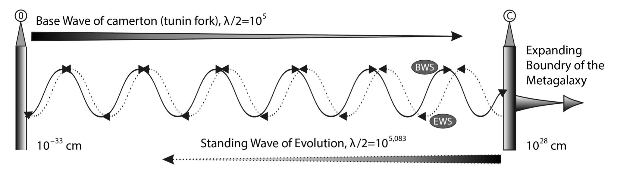Fig. 1.57. Characteristic stable points on the S-axis (dimensions) for the second wave - ESW depend on the radius of the Universe. As the Universe expands, the second sinusoid, unlike the first one (HLE), will stretch like an accordion to the right, and all the stable points it defines will also shift along the S-axis to the right

Then, for example, the coordinate (dimensions in fundamental length units) of the average human height on the S-axis will look like this: \(\lg D\) = 2.2 - (- 32.8) = 35. This shows that the "size" of a person is exactly 35 orders of magnitude larger than the size of the fundamental length.

Now let us choose a function for modeling the SWS, let us take the cosine function. Let us denote by a unit the state of ultimate stability of the system in each of the seven potential stability holes on the SWS. Accordingly, in the places where the cosine crosses the X-axis, its values will be equal to zero. Let us assign to it the value of the limit unstable state of the system. The upper points of the function will respectively take the value "minus 1", which will reflect their stable saddle equilibrium (see Fig. 1.58).

Recall that the stability vector in our SU model is directed downward, hence below the S-axis the function values are positive, and above the S-axis they are negative.

All these notions are very and very conventional since the concept of system stability itself has a complex and rather complicated meaning, which we will not discuss here. The introduction of these formalisms is necessary, first of all, to give the SWS a semblance of functional dependence and to be able to calculate the characteristic points on the S-axis using a formula rather than a ruler.

With the accepted notations, the SWS has the following functional form:

\[ F_0(L) = \cos\left(2\pi \cdot \frac{\lg D}{\lg 10^{10}}\right) = \cos(36° \cdot \lg D) \tag{1.13} \]

where \( F_0(L) \) is the basis scale stability function of the system, and \( 10^{10} \) is the dimensionless scale wavelength (meaning the length of the BASIS scale wavelength).

Calculation by formula (1.13) will allow us to find all the most characteristic dimensions and determine their rank by HLB.

Particular attention should be paid to the fact that at integer values: \( \lg D = N = 0, 1, 2, 3, 4, 5, 6... \), which characterize all points on the S-axis, going through the factor of increasing the size by a factor of 10 times, the function (1.13) takes values:

\[ F_0(L) = \cos(36° \cdot N) = 1, (0.809), (0.309), (-0.309), (-0.809), (-1), (-0.809),... \]

In the obtained series, in addition to the obvious, predetermined values 1 and -1, we find intermediate values of the function, which can be represented in another form:

\[ \pm 0.809 = \pm (0.5 \cdot 1.618), \] \[ \pm 0.309 = \pm (0.5 \cdot 0.618). \]

In the parentheses, we find two very important symmetry coefficients. One of them is the golden ratio (This fact was first brought to the author's attention by V. Komarov) and the other is equal to \({1}/{2}\).

As will be shown in the next book of the cycle, these two symmetry coefficients are the basis for two different types of symmetry: similarity and equality.

Consequently, the function we obtained takes a multiple of the golden ratio at the point between the two stability limit states on the S-axis.

What is the connection between WU and the famous golden ratio, it is difficult to say yet, but it is impossible to pass by this coincidence.

The stability function for the evolutional standing wave (ESW) has the following form:

\[ F_Э(L) = \cos \left(2\pi - \frac{\lg D}{\lg 10^{10.167}} \right) = \cos \left(35.4^\circ \cdot \log D \right) \tag{1.14} \]

That is, it is shifted in phase toward increasing the period on the S-axis by 0.167 units.

In the following, we will use this formula to determine the coordinate of the second mode \(X_Э\) on the S-axis:

\[ X_Э = \frac{1}{12}(r_В + 32.8) \cdot K - 32.8 \tag{1.15} \]

Where:

• \(X_Э\) is the exponent (power of 10) of the coordinate on the S-axis,
• \(K\) is the class number on the ESW,
• \(r_В\) is the exponent of the Universe’s radius at the time of interest (in cm).

Example:
Let the radius of the Universe be \(10^{28.2}\) cm. Then \(r_В = 28.2\). For Class #7, we get:

\[ X_Э = \frac{1}{12}(28.2 + 32.8) \cdot 7 - 32.8 = (12 \cdot 7 - 32.8) = 35.58 - 32.8 = 2.78 \]

This gives a characteristic size of \(10^{2.78}\) cm, or approximately 5 meters.

That means:
If the SWman (standing wave human) height is located on the S-axis at the HLB node with a coordinate of 1.6 meters, then five-meter giants (if they ever existed on Earth) would correspond to the HLB node at 5 meters on the S-axis.

You can write another formula to calculate the value of evolutionary fashion:

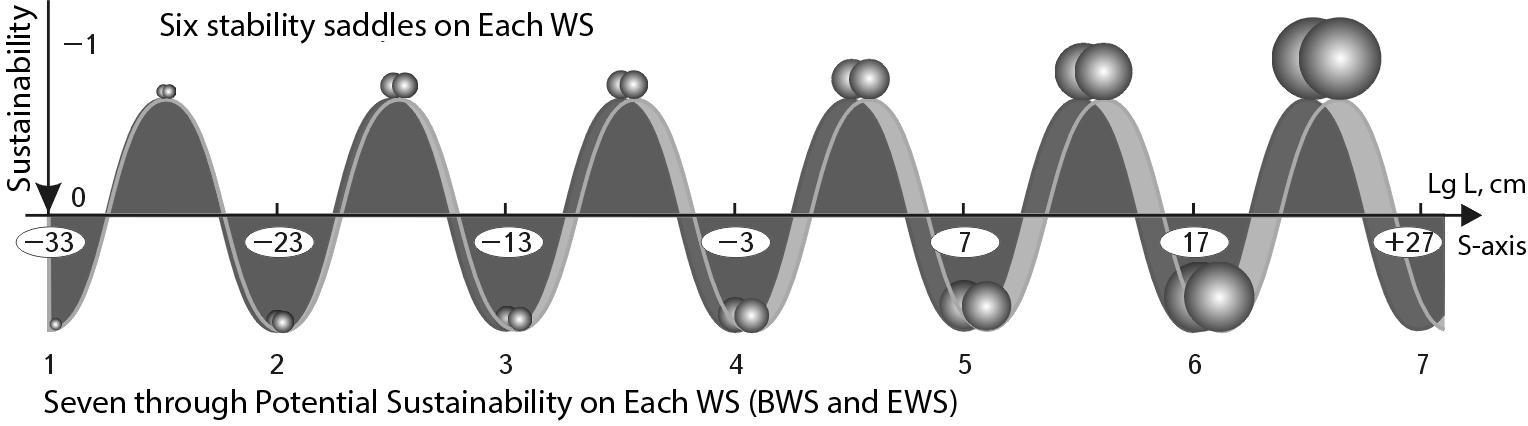Fig. 1.58. Model of two Waves of stability. At the top, on the crests of the SWS and EWS, there are the ranges of maximum stability sizes for the objects of the structural series - peculiar "stability saddles". At the bottom, in the seven troughs for SWS and EWS, there are zones of stable equilibrium for the objects of the nuclear series. The points of intersection of the EI with the S-axis are the points of maximum instability of objects

\[ L_K^{\mathbb{Э}} = l_f \left( \frac{R_B}{1_f} \right)^{K/12} \tag{1.16} \]

If we take the value \( R_B = 10^{27.2} \) cm, which corresponds to the scale-resonance state (approximately at the moment of its age of 1.6 billion years), then formula (1.16) will take the form that corresponds to the formula for calculating the basis first mode in the distribution on the SWS:

\[ L_K^{\acute{A}} = l_f \cdot 10^{5K} \tag{1.17} \]

We can verify the validity of the application of these modeling considerations by plotting the distribution diagrams of the main parameters of the main types of IS objects depending on their sizes, and then comparing the obtained mode values with the model values calculated based on two stability waves (see Fig. 1.57). Let us carry out such a comparison for the classes considered above.

NUCLEI OF ATOMS (CLASS #4). This is the first scale level from which we can rely on empirical data on the sizes of systems.

The first mode of the steady size according to SW is equal to
\[ 1.6 \cdot 10^{-13} \text{ cm} \]
(4 steps of 5 orders of magnitude from the point 0 – the fundamental length).
Let us repeat that the diameter of the most common particle in the Universe, the proton, has exactly this value.

The second stable size, determined based on the currently accepted size of the Universe of
\[ 1.6 \cdot 10^{28} \text{ cm} \]
according to the evolutionary formula (1.15), is equal to
\[ 10^{-12.47} \text{ cm} \approx 3.4 \cdot 10^{-13} \text{ cm} \]

The diameter of the second most common atomic nucleus in the Universe, the helium nucleus, is empirically determined from the geometry of its tetrahedral packing (see Figure 1.51).
It fits into a sphere with a diameter of
\[ 2 \cdot 1.6 \cdot 10^{-13} = 3.2 \cdot 10^{-13} \text{ cm} \]

Comparison of two values – model and empirical – shows a deviation of 6%. Taking into account the very approximate determination of the Universe radius at the present moment and as a consequence very approximate determination of the evolutionary coefficient of scale symmetry, the obtained result looks even too accurate.

We state that on the S-axis in the region of atomic nuclei on the basis of two SW the two most stable sizes are obtained: 1.6 and 3.4 fermi, which almost exactly correspond to the experimentally determined diameters of the two most stable nuclei and particles of the Universe (proton and α-particle).

However, this conclusion leads to a very serious contradiction with the whole cosmological theory. The matter is that the HW model is treated by us as a system of stable sizes allowed by nature.
At present, due to HLE, the stable existence of a nucleus with a size of about 3.4 fermi is allowed. If we go back in time, the value of the second stable point on the S-axis is less than 3.4 fermi.
This can be interpreted in such a way that before the age of the Universe of 10...12 billion years, helium could not be in a stable state. Simply put, it did not exist!

This contradiction can be partially removed if we PROPOSE that the tetrahedron of the helium nucleus has two stable dimensions:
the maximum is the diameter of the circumscribed sphere and the minimum is the height of the tetrahedron (see Fig. 1.52).

Calculation by formula (1.16) shows that at ESW the second mode reached the value of the minimum stable size, equal to 2.6 fermi for the α-particle, at an age of about 7 billion years.
Based on these models, we can reconstruct EVERYTHING that happened in the early universe.

Expanding to the right along the S-axis, the Metagalaxy has gradually shifted to the right all second modes of stable sizes since 1 billion years. For the first 7 billion years, this shift did not allow the helium nucleus to consolidate in a steady state.

However, after 7 billion years the shift reached the lower threshold of dimensional stability of the tetrahedral configuration of nucleons, which created preconditions for the continuous flow of hydrogen nuclei from the first mode of stability to the second one. The stormy process of the SECOND EPOCH of STRUCTURE-BREAKING began, in which the most favorable matrix-scale conditions were created for helium nuclei, which gave a start to the beginning of the mass synthesis of helium in the depths of stars. Since 7 billion years, these nuclei began to fall into stable spatial cells with sizes greater than 2.6 fermi and could be preserved in them for quite a long time.

Perhaps, it is these modeling considerations that lead to the explanation of the quiescence between the first and the second epochs of structure formation in the Universe.

Calculations with the SWS model show that the size range from the minimum size of the α-particle to the maximum second mode has passed in about 8–10 billion years of the Metagalactic expansion.
At present, the maximum size of the helium nucleus (\(3.2 \cdot 10^{-13} \text{ cm}\)) is slightly smaller than the value of the second mode of stability (\(3.4 \cdot 10^{-13} \text{ cm}\)) calculated by the formula (1.16).

ATOMS (CLASS #5). Once again, we recall that the calculated value for the first mode by SWS is \(1.6 \cdot 10^{-8} \text{ cm}\). The diameter of the hydrogen atom, according to the reference data, is \(1.4 \cdot 10^{-8} \text{ cm}\). The deviation is 13%, which is not so much if we take into account that the radius of the atom is empirically determined through the radius of the radial density maximum in the charge distribution of the neutral hydrogen atom. Clearly, beyond this radius extends some more space directly related to the hydrogen atom. It may extend just up to a diameter of \(1.6 \cdot 10^{-8} \text{ cm}\).

The evolutionary mode for the size distribution of atoms at a Metagalactic diameter of \(1.6 \cdot 10^{28} \text{ cm}\)
calculated by the formula (1.16), is \(4.1 \cdot 10^{-8} \text{ cm} \). We see (see Fig. 1.50) that the most significant mode in the size distribution of atoms (actual data) is noticeably smaller than \(\sim 3.0 \cdot 10^{-8} \text{ cm}\).

Several explanations are possible here.

First. Since the electron cloud does not have the same rigid structure as the nucleon droplets of nuclei, it can be secondarily affected by the nuclear characteristic sizes. They give rise in this case through the basis scale factor (\(10^5\)) of their twins:
1.6 and 2.4–3.6 angstroms (Fig. 1.59). The second range corresponds exactly to the width of the second model on the curve of the statistical distribution of atoms by size (see Fig. 1.49).

Second. It is possible that the size of the Metagalaxy is simply somewhat smaller, e.g. \(10^{28}\) cm. In this case, the evolutionary coefficient of scale symmetry will also be smaller. Consequently, the theoretical calculation will give a value closer to the real one.

Third. The second mode could have been generated by the second epoch of structure formation, which lasted from the age of 7 to 15 billion years. If we take the size of the Metagalaxy equal to \(7 \cdot 10^{27} \text{cm}\), then, using formula (1.16), we can obtain the coordinates of the second mode: \(10^{-7.53}\text{cm} = 2.9 \cdot 10^{-8} \text{cm}\), which is quite consistent with the value of the second mode in the distribution of chemical elements along the S-axis.

The model shows that the synthesis of atoms from the second mode mainly occurred during the second epoch of structure formation, and this is quite consistent with the astrophysical ideas about this process. Of course, this does not mean that the model imposes a ban on the synthesis of elements of this size class at the present time. It only means that the most rapid process of their formation coincided with the resonance state of the second epoch. The atoms of the second mode were preserved as a trace of this process. Now, probably, favorable is the SYNTHESIS OF THIRD MODE ELEMENTS, with the average diameter of atoms more than 4 angstroms, which corresponds to the weakly expressed third mode. Of course, we do not aim here to create a complete model of large-scale conditions for the process of synthesis of chemical elements during the expansion of the Universe. As we will show below, for more accurate calculation of all fine spectra of characteristic sizes it is not enough to involve simple logic of symmetry laws. Here it is necessary to apply in all its power the METHOD OF HARMONIC ANALYSIS. Only in this case it is possible to obtain a sufficiently accurate agreement with the available experimental data. But at the first stage, it is important to show the NEUTRALIZABILITY of the approach. After all, it is obvious that the statistical curve of atom size distribution clearly shows 2-3 modes, which are logically linked to 2-3 epochs of structure formation by means of simple translation along the S-axis of scale symmetry coefficients. Let us now evaluate to what extent the two-wave stability model allows us to obtain characteristic dimensions for stellar statistics. STARS. Since most modern stars are about 10 billion years old, they appeared around the second epoch of star formation and on average at the time of the expansion of the Metagalaxy, when it was about 7 billion years old. At that moment its dimensions were equal to 7 \(\cdot\) \(10^{27}\) cm = \(10^{27.85}\) cm. Let us determine by formula (1.16) the coordinates of the second mode for stars. They are equal to \(10^{12.69}\) cm.

Fig. 1.59. Conditional scheme of atom size distribution.

The values of the three modes (1.6; 2.6; 3.55 angstroms) can be obtained by relying on the dimensions of the proton and the helium nucleus (at the two extremes) by multiplying these dimensions by the constant \(10^{5}\).

Consequently, the characteristic size for stars of the second epoch of star formation has a degree index of 12.69. Observational data give a slightly smaller size of 12.45 (see Fig. 1.54), which corresponds to an age of the Universe of 3.4 billion years. For an age of 5 billion years, the coordinate on the S-axis would be 12.58. However, given the very approximate and averaged determination of the size of the Metagalaxy at the time when it was passing through the second epoch of violent star formation, the figures obtained by calculating the characteristic points of the SW can be considered satisfactory. It remains only to determine the characteristic size for the hypothetical third bell in the diagram (Sp-D), the bell that is populated by stars of the third epoch of star formation, the epoch that is going on now.

We determined the scale translation factor for the present-day size of the Metagalaxy earlier, it is equal to 5.083. The characteristic size for the stellar half-wave will be 12.95. The restoration of the third bell (see Fig. 1.54) shows that the sequence of bright giants is apparently an unfinished branch of the main sequence of the third epoch of star formation, which is in progress now. The coordinates of its top (12.9) are very close to the value obtained in our model. We can also predict the appearance of a branch of "new supergiants", which is probably represented only by very rare stars.

Now let us compare the first mode on the graph of atom size distribution with the first mode on the star diagram (Sp-D). We obtain that they are exactly 20 orders of magnitude apart: \(10^{12}\) cm : \(10^{-8}\) cm = \(10^{20}\) = (\(10^5\))^4, and to the nearest coefficient. The second stellar mode also correlates with the second atomic mode, only through a different coefficient - (\(10^{5.058}\))^4.

Concluding this section, we can state that the calculations using the two GPs of characteristic sizes on the S-axis for the stellar systems of the Metagalaxy do not contradict the available observational data, are logically consistent with them, and are confirmed in the main conclusions. Since our calculations use both free parameters and parameters not determined with sufficient accuracy, their correspondence to the actual data is certainly very approximate. But the logic of these calculations and the nature of the shift of the second mode as the class increases on the SW model are consistent.

So, our PROPOSAL about the role of integer symmetric divisions of the S-axis finds its very convincing confirmation. On the S-axis interval, as a space closed (by phase transitions) from both sides, with a length of 61 orders, exactly 12 times half-waves (or 6 times waves) of stability are arranged, generating a spectrum of stable dimensions every 5.083 orders, starting from any point (right or left). On the same S-axis we also find characteristic dimensions generated by another integer quantity, \(10^{5}\). It generates every 5 orders of magnitude its stable and characteristic dimensions, but they start from the left, and by the end of the interval there is a "tail" of one order on the right.

This "tail" at first sight spoils the whole integer symmetry. However, we remind that at the moment of the Universe expansion, when it reached the size of 1.6 \(\cdot\) \(10^{27}\) cm, the basis coefficient was exactly 12 times within the length of the whole S-interval, and there was no "tail". It was in this scale-resonance period that the first turbulent epoch of structure formation took place.

If we now depict the two stability waves side by side, we get a new picture of the MASTER HARMONY. We see a split spectrum of characteristic sizes along the whole S-interval. Consequently, any basic characteristic size in the Universe has another larger size standing next to it like a shadow. THUs, although the modes are very close, the sources of their stability are at opposite edges of the S-Interval of the Universe. The first mode is generated by the HLB, which "chamber tone" sounds from the left edge of the S-interval. The second mode is generated by the HEV, which is reflected from the right edge of the S-interval and forms a standing scale wave. THUs, very different, extremely different systems always "live" side by side in each of the classes, like INH and YAN.

Of course, if our model is correct, there can be no exceptions to this rule for any class of systems. We can speak in this case about GLOBAL BIMODALITY (multimodality) in the distribution of all kinds of systems of the Universe, which is determined by the harmonic interaction of the two main stability waves.

To test this assumption, we have chosen a level intermediate between the atomic and stellar levels - the scale level \(10^4\)-\(10^{10}\) cm. This choice is because in this size range one can find sufficiently representative information on some types of systems with stable sizes for a long time, and the number of which on the Earth, due to their scale, is small, which allows us to make a complete statistical sampling.